Understanding Backpropagation

Backpropagation is arguably one of the most important algorithms in all of computer science. It’s certainly the most important in neural networks and deep learning. Unfortunately, many students don’t really understand what it is, why it is needed, or what it actually computes. There seems to be two prevalent types of explanations: the super-high-level, hand-wavy one and the “boards and boards of equations” one. In reality, these are really two different views of the same thing. Having a solid understanding of backpropagation means you can explain it in both of these ways. My goal is to provided an alternate explanation of backpropagation that’s sandwiched right in between these two views.

Many students treat backpropagation and training of neural networks as some mystic black-box where you provide some input and ground-truth data and the machine does some magical computations. Backpropagation is actually much simpler than most students think it is.

Backpropagation is simply a direct application of the chain rule

I’m also going to use concrete examples. When learning a new topic (or familiarizing yourself with an old one), abstractness can be the enemy here. I’ve found that starting with intuition and examples tends to help students learn better than starting with abstract definitions and general cases. Of the students that do know backpropagation, most only learned it abstractly and have never coded it or performed it by hand. Doing even one example by hand can help greatly improve understanding.

Let’s get started!

First, we have to understand why we need backpropagation in the first place. Consider a single layer neural network:

\[\begin{aligned} z &\equiv Wx + b\\ a &\equiv \varphi(z) \end{aligned}\]

where $\varphi$ is a sigmoid ($\varphi(z) = \frac{1}{1+\exp(-z)}$). Conventionally, we call $z$ the weighted sum or pre-activation and $a$ the post-activation or simply the activation. For our example, suppose that $W = [2~~~-3]$ and $b = -3$. In practice, our weight matrix is initialized to small, random values to break network symmetry, and our biases are initialized to zero.

To train our weights and biases, we need to come up with some measure of how well it’s doing. For example, we could use the quadratic cost.

\[C(y, a) = \frac{1}{2}\sum_{i=1}^N (y - a)^2\]

The cost/loss/error function is always a function of the ground-truth output and the output of the network, i.e., the last layer. With all of this information, we can compute a forward pass for a particular input. For our running example, our input vector will be $x=[-1~~~-2]^T$, and the target output for $x$ will be $y=1$. We can perform a forward pass and feed our input vector through the network to compute the network’s output.

Computation Graphs

Visually, we can represent this single-layer network as a computation graph (where the components of the weights are explicitly shown).

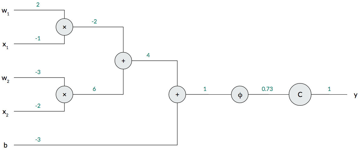
A computation graph is just a collection of operations that takes some input, performs some processing, and produces some output, just like a mathematical function. This is one way of interpreting a neural network: the network just computes a function parameterized by the weights and biases. The computation graph above shows a single-layer network, but we could easily add more nodes to extend this to a multi-layer network.

For our example, I’ve filled in all of the intermediate computations in green above the edges connecting the operations. In our example, the correct answer is $1$, yet our network produces $0.73$. This produces a loss of $(1-0.73)^2=0.0729$ for this example. Our network could do better, so let’s train it.

Gradient Descent

Recall that we usually use gradient descent (or some other variant) to train our network. The update rule of gradient descent, for some parameter $\theta$, is always the following.

\[\theta \gets \theta - \alpha \frac{\partial C}{\partial\theta}\]

(Technically, $\frac{\partial C}{\partial\theta}$ isn’t a gradient, but, in practice, we use vectorized implementations of gradient descent, which is why I’ll still refer to $\frac{\partial C}{\partial\theta}$ as a gradient.)

In words, to update a parameter, we compute the partial derivative of the cost function with respect to that parameter and nudge the parameter in the opposite direction. We use a learning rate to scale this nudge, and there are much fancier ways of annealing the learning rate. Intuitively, to perform gradient descent, we need to quantify the contribution of each trainable parameter to the overall cost. This is also why backpropagation is sometimes called backpropagation of errors: if we have a nonzero loss, each trainable parameter is to blame! Computing the partial derivative allows us to quantify that blame. As my calculus professor once said, “the partial derivative tells you how [$C$] will wiggle if you wiggle [$\theta$].” After computing the partial derivative of the cost function with respect to each parameter, we update the parameters, according to gradient descent, to try to decrease the overall cost.

Backpropagation Example

Getting back to our example, we have three trainable parameters: $w_1$, $w_2$, and $b$. Following gradient descent, we need to compute three partial derivatives: $\frac{\partial C}{\partial w_1}$, $\frac{\partial C}{\partial w_2}$, and $\frac{\partial C}{\partial b}$. There’s just one huge issue with computing the partial derivative of the cost function with respect to $w_1$, $w_2$, and $b$: the parameters are not directly in the cost function! Take a look at $C$ again. There’s no $w_1$, $w_2$, or $b$ anywhere.

However, the cost function does have the output of our network $a$, which is a function of $z$, which is a function of $w_1$! Jackpot! We can chain together these using the chain rule of calculus! Always remember that backpropagation is really just a direct application of the chain rule.

\[\frac{\partial C}{\partial w_1} = \frac{\partial C}{\partial a}\frac{\partial a}{\partial z}\frac{\partial z}{\partial w_1}\]

Notice that each function in the numerator is a function of the variable in the denominator. Now all that’s left to do is compute these partial derivatives and plug in values! Let’s start with the outermost partial derivative:

\[\begin{aligned} \frac{\partial C}{\partial a} &= -(y-a)\\ &= -(1 - 0.73)\\ &= -0.27 \end{aligned}\]

Now we have to compute the partial derivative of the output of the sigmoid with respect to the input of the sigmoid. Luckily, the sigmoid has an easy derivative. Also, notice that $a\equiv\varphi(z)$, so a substitution saves us a computation.

\[\begin{aligned} \frac{\partial a}{\partial z} &= \varphi(z)[1-\varphi(z)]\\ &= a(1-a)\\ &= 0.73\cdot(1-0.73)\\ &= 0.1971 \end{aligned}\]

Finally, we have to compute the partial derivative of the weighted input with respect to the actual parameter $w_1$.

\[\begin{aligned} \frac{\partial z}{\partial w_1} &= x_1\\ &= -1 \end{aligned}\]

Finally, we can multiply everything together to get the partial derivative of the cost function with respect to $w_1$! This is the value we use for updating $w_1$ with gradient descent.

\[\begin{aligned} \frac{\partial C}{\partial w_1} &= \frac{\partial C}{\partial a}\frac{\partial a}{\partial z}\frac{\partial z}{\partial w_1}\\ &= -0.27\cdot 0.1971\cdot -1\\ &= 0.053217 \end{aligned}\]

Congratulations! You just performed backpropagation by hand! It wasn’t that bad, was it?

For fun, let’s take a look at applying the chain rule for the other weight $w_2$.

\[\frac{\partial C}{\partial w_2} = \frac{\partial C}{\partial a}\frac{\partial a}{\partial z}\frac{\partial z}{\partial w_2}\]

This seems awfully familiar. In fact, the first two factors of the product are exactly the same factors when we were computing $\frac{\partial C}{\partial w_1}$. Why compute them again? We usually define an intermediate variable $\delta$ that represents the error gradient at a layer (or the layer, in our case).

\[\delta \equiv \frac{\partial C}{\partial a}\frac{\partial a}{\partial z}\]

Now we simply compute $\delta$ once and multiply it by $\frac{\partial z}{\partial w_1}$ or $\frac{\partial z}{\partial w_2}$. But what about the bias?

\[\begin{aligned} \frac{\partial C}{\partial b} &= \frac{\partial C}{\partial a}\frac{\partial a}{\partial z}\frac{\partial z}{\partial b}\\ &= \delta\frac{\partial z}{\partial b}\\ &= \delta\cdot 1\\ &= \delta \end{aligned}\]

The bias is exactly equal to the error gradient $\delta$! This is process of computing the partial derivatives backward through the network is also why one “step” of backpropagation is sometimes called the backward pass.

Backpropagation in Computation Graphs

Like with the forward pass, we can show the backward pass in our computation graph. We can represent it in our computation graph very intuitively: we travel backward from the cost function to the parameters.

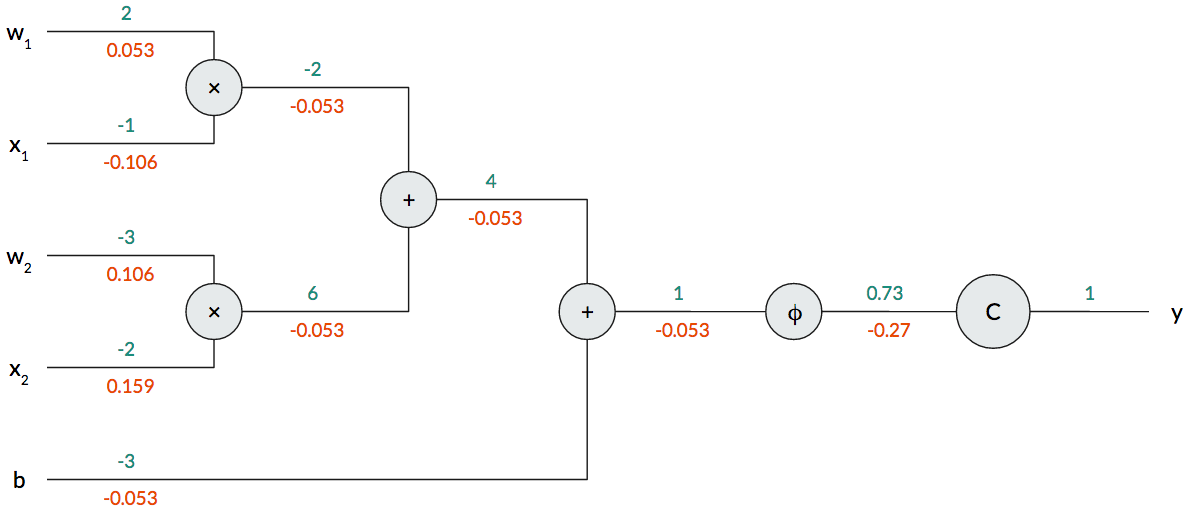
When computing backpropagation using a computation graph, we compute the “local gradient” and multiply that with the incoming gradient. Take a look at the $\varphi$ operation node. Above, we computed local gradient to be $0.1971$. We multiply this with the incoming gradient $-0.27$ to get $-0.053$. We keep doing this as we progress backward through the graph. Eventually, we’ll arrive at the parameters and inputs. Since the inputs aren’t trainable (in this case), we only consider the parameters $w_1$, $w_2$, and $b$. After running backpropagation, we’ve computed the value of the gradient for each parameter with respect to the cost function.

Now we can perform gradient descent. To illustrate that we do get a smaller loss value with gradient descent, let’s update the parameters with $\alpha=1$. This learning rate is way too large to use in practice, but it works well for our small example. Our new parameters are $w_1=1.94, w_2=-3.106, b=-2.947$, and, if we compute a forward pass using the same input but these new parameters, we get an activation of $0.79$, which is closer to our target value of $1$! Backpropagation really works, even in small examples by hand!

Properties of the Gradient in Computation Graphs. Let’s go back to the computation graph. We notice some interesting characteristics of the gradient as it progresses backward through the nodes that give us some insight on how different operations affect the gradient. For example, consider what happens to the gradient at the addition operation node: it copies! For the multiplication gate, we perform a kind of “scaled switch” where we multiply the gradient by the opposite value. Mathematically, $\frac{\partial z}{\partial w_1}=x_1$ and $\frac{\partial z}{\partial x_1}=w_1$.

Using the computation graph shows that backpropagation is more general than just neural networks. Although backpropagation was invented specifically for neural networks, its underlying concept, the chain rule, can be applied for any computation! That what makes backpropagation so powerful! But this same beauty also makes backpropagation dangerous: students often use a deep learning library, e.g., Tensorflow, PyTorch, etc., and think “well I don’t have to know about backpropagation since the automatic differentiation will just train anything I code up.” This kind of thinking gets us into trouble when we try to train deep models.

Backpropagation in Deep Neural Networks

We’ve only seen backpropagation applied to a single-layer neural network. What about deep neural networks with many hidden layers? Backpropagation becomes a bit more complicated, but it’s still the same principle: apply the chain rule! Really nothing else changes except we have more factors, i.e., partial derivatives, when we use the chain rule to compute the partial derivative of the cost function with respect to a particular weight or bias.

However, the danger of not understanding backpropagation becomes very evident when we discuss deeper networks: we can’t simply stack layers and layers on top of each other and expect backpropagation to magically work. If you had the mindset of “Tensorflow/PyTorch will automatically do backpropagation for me so I don’t have to learn it”, then you’re in for a real shock when you try to train deeper networks.

Vanishing Gradient. The biggest issue impeding network depth is the vanishing gradient problem. This is a direct result of backpropagation and the activation function we choose. Remember that we’re just applying the chain rule at each layer, multiplying quantities together in a long string. If each factor is smaller than one, the product of those factors is going to be very close to zero. This is not good for learning! By the time we reach the earlier layers, there’s no gradient to use for training!

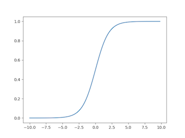
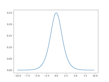
This problem is exacerbated by the sigmoid and tanh (hyperbolic tangent) activation functions. The sigmoid and its derivative are shown below.

The tanh activation function and its derivative are shown below. Notice the tanh is really just a scaled sigmoid ($\tanh(x) = 2\varphi(2x)-1$).

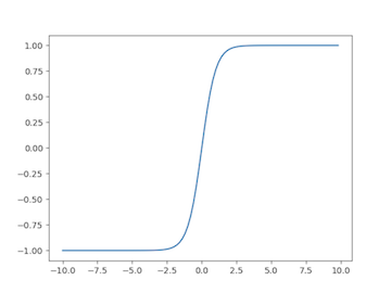
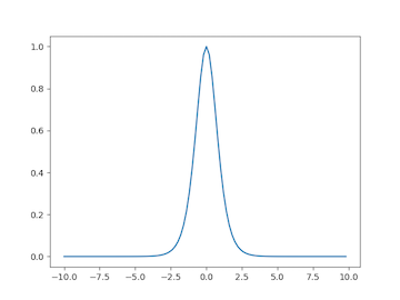
When we use backpropagation, we’ll be multiplying the gradient by the derivative of the sigmoid or tanh evaluated at the weighted sum input, i.e., $\varphi’(z)$. But take a look at the derivative of the activation functions: many values of $z$ produce to an output close to zero. There are only a few values near zero where the output of the derivative is greater than zero. We say the neuron has saturated if the local gradient is close to zero, which happens when the weighted sum $z$ is large in magnitude. This inhibits gradient retention as we go backward through our network. In other words, we don’t have as much gradient to share when we get to the weights in the earlier layers. The update rule for the weights is a function of the incoming gradient, and this causes our weights to update very slowly. Hence, our network converges very slowly.

If we have a very deep network, we’re backpropagating through many of these activation functions, and our gradient keeps getting smaller and smaller. By the time we reach the first few layers’ weights, the gradient is almost zero! Therefore, these weights don’t get updated to the same degree as the weights further in the network.

ReLU Neurons. One solution to this problem is to design a new activation function that doesn’t saturate. For example, the rectified linear unit (ReLU) activation function doesn’t have this issue of saturation. The ReLU is defined with a max operation $\varphi(z)\equiv \max(0,z)$. Take a look at a plot of the ReLU and its derivative, shown below respectively.

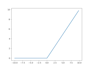
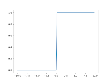
How does this prevent saturation? The issue with the sigmoid and tanh is that the derivative value will be less than one, grinding the gradient down to zero. However, with the ReLU, the derivative is simply one if the weighted sum input is greater than zero. Thinking of it as a chain of factors, many of the products will simply be one. Multiplying the incoming gradient by one doesn’t do anything to it, and we preserve the gradient through this activation function!

Success! Right? Not quite. It has its own issue: dying ReLUs. If the input to the ReLU is less than zero, the incoming gradient is zeroed out as we try to backpropagate through a ReLU neuron. If a weight update causes the weighted sum input to be negative, then this neuron is effectively killed, permanently.

One solution is to use a leaky ReLU: instead of a max, use a piecewise function that has some small negative value if the input is less than zero. When computing the derivative, it will be a small value rather than exactly zero.

Exploding Gradient. There is a complimentary problem called exploding gradient that occurs commonly in recurrent neural networks (RNNs). As the name implies, instead of the gradient going to zero, the gradient explodes toward infinity. But why is this a problem? Computationally, the gradient will chomp through the bits in a 32 or 64-bit floating-point number, and overflow errors are very common and a clear indicator of exploding gradients! With RNNs specifically, this means the network has difficulty with long-term dependencies and relationships. To see why this happens, take a look at an “unrolled” vanilla RNN below.

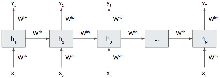
Different from a plain neural network, we evaluate the cost function at each time step (in the above RNN). When we backpropagate through an RNN, we “unroll” it for a fixed number of time steps. Each unrolled unit is essentially a deep neural network with shared weights across time. Intuitively the network is trying to retain more information to remember. As we keep trying to add more and more information to the gradient, it tends to explode toward infinity.

The simplest solution here is to clip the magnitude of the gradient (between -5 and 5 works well). But that doesn’t really solve the problem; it just sidesteps it. Instead, variants of the vanilla RNN have been invented, such as the long short-term memory (LSTM) cell and gated recurrent unit (GRU), that are always used in practice over the vanilla RNN. These variants have additional “gates” and operations that help the gradient flow better without vanishing or exploding.

For example, an RNN that uses LSTM cells rarely experiences vanishing or exploding gradient. To counteract vanishing gradient, the “recurrent” part of the LSTM cell is a sum; thus the gradient is simply one, and multiplying the gradient by one doesn’t change it. To counteract exploding gradient, there is an additional operation, called the forget gate, that is applied, component-wise, to the internal cell state and is never greater than one. This helps scale back the gradient at each time step, preventing it from exploding.

It should be noted that non-recurrent networks can still suffer from exploding gradient, but it’s much less common than vanishing gradient. The moral of the story is that understanding backpropagation helps you identify issues in your network such as vanishing and exploding gradient.

Conclusion

Backpropagation is not magic; it’s math. Specifically, backpropagation is just an application of the chain rule many times. Knowing how backpropagation works under-the-hood will help you better train and debug your neural networks.

I’ve relied on your intuition when explaining backpropagation. When I was first learning it, it was enough to whet my appetite, but I grew hungry for a deeper, more mathematical understanding. If you’re looking for that, Michael Nielson has a fantastic post here that derives and describes the mathematical formulation of backpropagation.

If you learn one thing from reading this post, remember that backpropagation is just a direct application of the chain rule!