Deep Reinforcement Learning: Value-based Methods
In my previous post on reinforcement learning, I explained the formulation of a game and a way to solve it called a Markov Decision Process (MDPs). However, MDPs are useable only when we know which transitions lead to which rewards; in many real-world scenarios and games, we don’t have this a-priori knowledge. Instead, we can repeatedly play the game over and over again to learn which actions in which states lead to the highest expected reward. This algorithm, called Q-learning, is the basis for reinforcement learning.
However, it’s just the tip of the iceberg: researchers have incorporated neural networks into reinforcement learning to create deep reinforcement learning architectures that are capable of winning against humans at more advanced games such as Go, Atari games, and DOTA. In this post, we’re going to look at a category of deep reinforcement learning algorithms, called value-based learning, that derive the best policy using q-values.
For a more concrete understanding, i.e., code, I have a repo where I’ve implemented the DQN models and algorithms of this post in Pytorch.
Approximate Q-learning
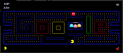
Credit: Pacman Doodle. May 21, 2010. google.com
To motivate our discussion of deep reinforcement learning, let’s consider a game that is marginally more complicated than our GridWorld game: PacMan. The premise of the game is similar: maximize the score by eating pellets and avoiding ghosts. The entities are PacMan, the ghosts and their various states (normal, flashing, etc.), and the pellets. Hence, a complete state would include the location of PacMan, the locations of all of the ghosts, the states of all of the ghosts, and the locations of the remaining pellets. With some thought, we might be able to merge some elements of the state space into one entity, but, overall, we have a very large discretized state space!
Performing vanilla Q-learning on this state space will create a massive q-value table with many states, and itʼs very unlikely that we’ll reach each state during training. At this point, we may even run into memory issue storing this massive q-value table!
One technique to alleviate this large state space is called Approximate Q-learning. Instead of storing state-action information in a large q-value table, we represent the q-value as a weighted sum of feature functions that convert the raw state into values important to our agent. For example, we could write a feature function that returns the number of pellets PacMan has left to eat or the position of the nearest ghost using Manhattan distance. We hand-design a number of these feature functions $f_1(s, a), \dots, f_n(s, a)$ and associate trainable weights $w_1, \dots, w_n$. Our new q-value function looks like the following.
\[Q(s,a) = w_1 f_1(s, a) + \dots + w_n f_n(s, a)\]In other words, given a state $s$ and action $a$, we compute the q-value by taking the weighted sum of our feature functions.
Intuitively, the weight of a feature function is increased if that feature tends to produce better results and vice-versa for feature functions that lead to poor results. Given a transition $(s, a, r, s’)$, this results in the following update rule for the weights:
\[w_i \gets w_i + \alpha (r + \gamma \max_{a'} Q(s', a') - Q(s, a)) f_i(s, a)\]Compare this to the update rule for Q-learning:
\[Q(s, a) \gets Q(s, a) + \alpha (r + \gamma \max_{a'} Q(s', a') - Q(s, a))\]The first difference is we’re learning the weights in order to compute the q-values; we’re not computing the q-values directly. We multiply the feature function $f_i(s, a)$ to learn which features tend to produce higher scores. Incorporating these feature functions into the weight update allows our agent to learn which features in which states help maximize the score.
Using Approximate Q-learning in place of vanilla Q-learning can help improve our agent’s generalization ability by using weighted sum of hand-tailored feature functions to represent a state rather than the state itself. The result is we see better performance on games with larger state spaces such as PacMan.
Deep Q-Networks (DQNs)
Approximate Q-learning has a major flaw: the quality of the agent is dependent on the user-defined feature functions. Writing good feature functions will produce an intelligent agent; there’s a bit of trial-and-error involved in determining which feature functions produce an intelligent agent. However, as with the vision community and its handmade feature detectors for images, we can replace the feature functions with a neural network that will compute the q-value function $Q(s, a)$.
This neural architecture is the premise of deep reinforcement learning and the Deep Q-Network (DQN). The basic design of DQNs is quite simple: the input is a raw image of our game, and the output is a q-value for each action.
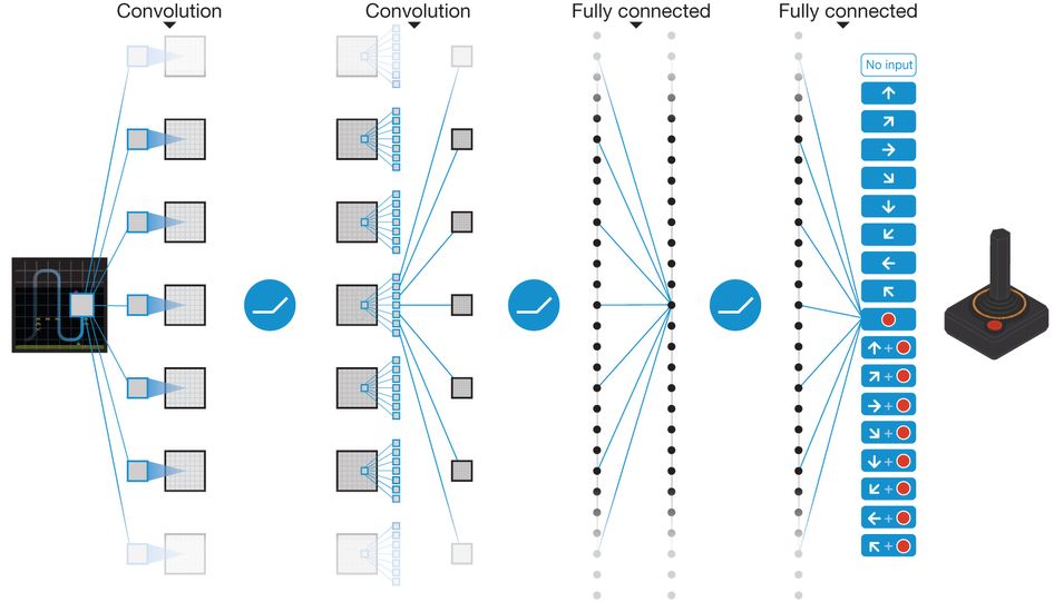
Human-level control through deep reinforcement learning by Mnih et al.
We can replace the feature functions with this neural network and devise the most fundamental DQN training algorithm. Since we’re using a neural network, we train the weights using gradient descent on the temporal difference error (also called the Bellman error).
Here is the fundamental DQN training algorithm.
- Initialize DQN $Q(x, a)$
- For each episode do
- For each step do
- In frame $x_t$, with probability $\epsilon$, take a random action, else take best action $a = \arg\max_{a’} Q(x_t, a’)$
- Execute action $a$ to receive reward $r$ and next image $x_{t+1}$
- If end of game, compute the q-value $y = r$
- If not end of game, compute q-value $y = r + \gamma\max_{a’}Q(x_t, a’)$
- Perform gradient descent on step using the quadratic loss of the temporal difference error $(y - Q(x_t, a))^2$
- End For
- For each step do
- End For
(This algorithm takes an online approach, but we’ll soon see how to batch our data when we discuss experience replay.)
As an example, let’s consider the classic Atari game of Breakout.
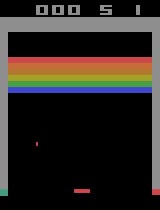
Credit: OpenAI Gym.
The goal of the game is to break all of the bricks with the ball without dropping it. Our states are now frames of the game, and our possible actions are move a little to the left, move a little to the right, and do nothing. The reward is simply the score of the game. We feed the frame into the DQN, and it produces q-values for each action. Then we simple select the action with the largest q-value, just like with Q-learning.
While DQNs essentially replace the weighted sum of the feature functions, vanilla DQNs are very difficult to train because they have many convergence issues. To get DQNs to work well in practice, we must make several key modifications to the learning algorithm.
Frame Stacking, Skipping, and Processing
The first improvement we can make is to process the input. In particular, we can give our DQN some notion of velocity and motion by stacking several frames together. Think of the Breakout game: if we look at several consecutive frames, there’s the motion of the ball and the paddle. Hence, we can stack several frames into a single tensor and feed that as an input to our network. In the case of Breakout, suppose we wanted to stack 4 frames of size $84\times 84$ together. Then the input to our network would be a 3-tensor of size $84\times 84\times 4$.
As an example, we take only every fourth frame and stack those together into a single observation input to our DQN. These skipped frames give our DQN a better perception of velocity and motion in our game.
However, we don’t quite stack 4 consecutive frames together. Instead, we skip frames. The reason we do this is to prevent our network from making strong correlations about the states immediately before it. Another reason is to give our DQN a more useful sense of motion: the ball and paddle won’t move much between two consecutive frames in a game like Breakout. To fully conceptualize the idea of motion and velocity, we skip frames before we stack them.
(To be thorough, there’s an additional step that Google DeepMind used in their Nature article on deep reinforcement learning: they took the max between a frame of the input and the skipped frame immediately before it. This step was added because of how Atari renders sprites.)
Experience Replay
Another improvement on vanilla DQNs is called experience replay. Instead of training our network on sequential frames of video, we store all of the state transitions $(x_t, a_t, r_t, x_{t+1})$ into a replay memory. Under the hood, this may be implemented as a ring buffer or any data structure with fast sampling and the ability to replace old transitions with newer ones.
After storing transitions into the replay memory, at each step, we randomly sample a mini-batch and compute the q-value for each transition in the mini-batch under the current parameters of our DQN. Then we perform a gradient descent step on the mini-batch with the target q-values and update the DQN’s parameters for the next step.
In practice, we don’t start training the DQN until our replay memory is full so the first few thousand or hundred thousand or million transitions aren’t actually used to train the network: they fill the replay memory by taking random actions. After we have a full replay memory, we can sample mini-batches from it to train our network. As we collect more transitions, we replace the old transitions in the replay memory with these newer ones which is why a cyclical data structure is used for the replay memory.
Why do we need experience replay? It can greatly improve generalization by minimizing correlations in our training data. Sequential frames of the game are highly correlated, and we do not want our network to learn these tight correlations in the sequence of gameplay frames. By storing these transitions and randomly sampling, we force our DQN to make the best decision based only on the stack of frames it receives, with no other a-priori information to help it.
Target Network
The final improvement on vanilla DQNs, at least by the original paper, is incorporating a target network $\hat{Q}$. We’ll call the original DQN $Q$ the online network since we now have two networks. The target network is a copy of the online network and is used to compute the q-values for each transition in the mini-batch. The online network is used to compute the best action, and only its weights are updated via gradient descent. The target network’s weights are set to the online network’s weights at some number of time steps $C$. In other words, the target network’s weights are copied over from the online network every $C$ steps.
The purpose of the target network is to add stability. Consider what happens to the online network as we train: its weights are frequently being changed, and, consequently, the resulting q-values from that network will also frequently change and so on and so on. By using the target network to compute the q-values and updating its weights less frequently, we have more stable q-values, and our online network trains quicker.
Reward Clipping and Huber Loss
There are a few minor improvements that we can make to help improve the stability of training for our DQN. One improvement is to clip the rewards to $[-1, 1]$. This prevents extreme outcomes from affecting our DQN, causing the weights to jump drastically.
Similarly, we can clip the gradients to $[-1, 1]$ as well to prevent a weight update from being too large. However, an even better way to do this is to use the Huber Loss instead of the quadratic loss.
\[\mathcal{L}_\delta(t) = \begin{cases} \frac{1}{2}t^2 & \vert t\vert\leq \delta \\ \delta(\vert t\vert -\frac{1}{2}\delta) & \mathrm{otherwise} \end{cases}\]A plot of this function is shown below.
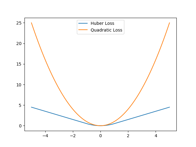
Small inputs act quadratically for the Huber Loss while large inputs act linearly. In either case, the magnitude of the derivative is never greater than 1.
(We usually set $\delta=1$.) For small values, Huber Loss is quadratic, and, for large values, Huber Loss acts linearly. Intuitively, for small temporal difference errors, we use the quadratic function, but, for large errors, we use the linear function. Notice that the gradient of the Huber Loss is never greater than one!
DQN Training Algorithm
After incorporating the frame skipping and processing, experience replay, and target network, the final DQN algorithm becomes the following.
- Initialize replay memory $M$
- Initialize online network $Q$
- Initialize target network $\hat{Q}$
- For each episode do
- For each step do
- Create a sequence $s_t$ from the previous processed frames
- With probability $\epsilon$, take a random action, else take best action $a_t = \arg\max_{a’} Q(s_t, a’)$
- Execute action $a_t$ to receive reward $r_t$ and next image $x_{t+1}$
- Process $x_{t+1}$ and incorporate it into a frame sequence $s_{t+1}$
- Store the transition $(s_t, a_t, r_t, s_{t+1})$ into the replay memory $M$
- Sample a random mini-batch of transitions $(s_k^{(j)}, a^{(j)}, r^{(j)}, s_{k+1}^{(j)})$ from $M$, where each transition in the mini-batch is indexed by $j$.
- Clip all rewards $r^{(j)}\in [-1,1]$
- If end of game, set q-value to reward: $y^{(j)} = r^{(j)}$
- If not end of game, set q-value using target network: $y^{(j)} = r^{(j)} + \gamma\max_{a’}\hat{Q}(s_{k+1}^{(j)}, a’)$
- Perform a gradient descent update of the online network using the Huber Loss of the temporal difference error $\mathcal{L}_1(\mathbf{y} - Q(\mathbf{s_k}, \mathbf{a}))$.
- Every $C$ steps, update the target network’s weights $\hat{Q}=Q$
- End For
- For each step do
- End For
This is the same algorithm and approach used by DeepMind in their seminal paper on deep reinforcement learning. The implementation of this training loop is in my repo here.
Double DQN
Even with those improvements to the vanilla DQN algorithm, DQNs still have a tendency to overestimate q-values because the same network selects which action to take and assigns the q-value, leading to overconfidence and subsequently overestimation.
Mathematically, the issue lies in the function we use to set the q-value:
\[y = r + \gamma\max_{a'}\hat{Q}(s', a')\]However, in the beginning of training, our DQN doesn’t know which action is the optimal action, and this causes our DQN to assign high q-values to non-optimal actions. Then, our agent will prefer to take these non-optimal actions because of those high q-values, and training becomes more difficult because our agent needs to “unlearn” those non-optimal actions.
The solution is to split up this q-value estimation task between the online and target networks. The online network $Q$, with the latest set of weights, i.e., the greedy policy, will give us the best action to take given our state $s’$, and the target network $\hat{Q}$ can fairly evaluate this action to compute the q-value. Through this decoupling, we can prevent overoptimism.
The only change we have to make is how we compute the q-value:
\[y = r + \gamma\hat{Q}(s', {\arg\max}_a Q(s', a))\]The online network computes the best action using a greedy policy while the target network fairly assesses that action when it computes the q-value. This minimal change produces more stable learning and a significant drop in training time.
If this explanation of separating the estimation between the online and target networks isn’t convincing enough, the original paper has proofs that compute overoptimism and its bounds regarding the vanilla DQN algorithm and the double DQN algorithm.
Dueling DQN
The Dueling DQN takes a different approach to the DQN model. First, we define a quantity called advantage that relates the value and q-value functions.
\[A(s,a) = Q(s, a) - V(s)\]Intuitively, the value function tells us how good it is to be in state $s$, i.e., the future expected reward of being in state $s$. The q-value tells us how good it is to take action $a$ in state $s$, i.e., the expected reward of taking action $a$ in state $s$. Hence, the advantage function tells us how much better it would be to take action $a$ in state $s$ over all other possible actions $a\in\mathcal{A}$ in state $s$.
Using this definition of the advantage function, we can rewrite the q-value function as the following.
\[Q(s, a) = V(s) + A(s, a)\]There are a few interesting equations that follow from our advantage function definition and knowledge of value and q-value functions that will help us better understand the advantage function and the Dueling DQN model.
Suppose we have an optimal action $a^\ast=\arg\max_{a’\in\mathcal{A}}Q(s, a’)$. Then $Q(s, a^\ast) = V(s)$ (for a deterministic policy) because taking the best action in any state is equivalent to that state’s value, i.e., expected reward. By substituting that equivalence into the advantage function, we see that $A(s,a^\ast) = Q(s, a^\ast) - V(s) = 0$. Intuitively, the advantage of our action is 0 because we’re already taking the best possible action so any other action will produce an expected score worse than our value. Keep this in mind because we’ll revisit this notion soon.
With our q-value function written as the sum of the value and advantage function, we can devise an architecture that learns these two terms separately.
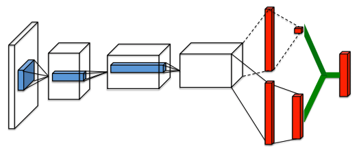
Dueling Network Architectures for Deep Reinforcement Learning by Wang et al.
Dueling DQNs split our network into two branches: the top branch that compute the value of the state and the bottom branch that computes the advantage for each action. Then, the two branches are merged again to produce the q-values.
The immediate question you might ask is “what’s the point of splitting the branches if we’re just going to combine them at the end?” We split the value and advantage so we can learn about good states without necessarily learning about the actions in those states.
The Dueling DQN paper has a good example: imagine a car driving game where the objective is to go as far as we can without crashing. If the road ahead is completely empty, action of moving out of the way is irrelevant. On the other hand, if there are cars in front, the action we take is critical to the score, i.e., we want to avoid driving into other cars!
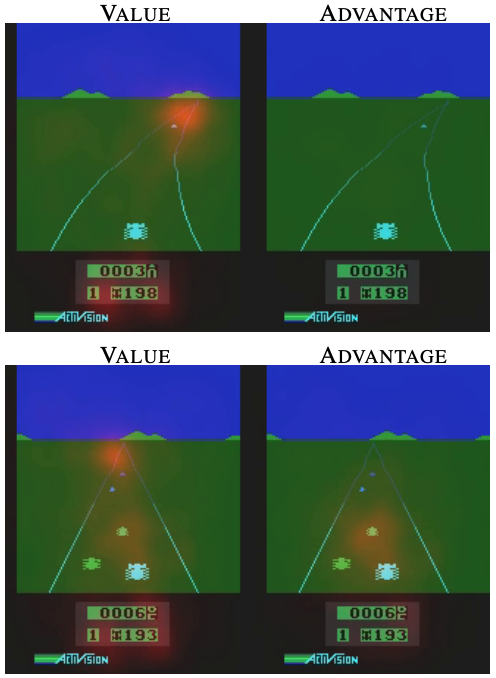
Dueling Network Architectures for Deep Reinforcement Learning by Wang et al.
The saliency maps of the two streams are shown as an orange overlay. Notice that the value stream learns to attend to the road itself, and the advantage stream only pays attention when there are cars immediately in front of our driver.
By splitting the q-value into the value and advantage, we can compute the value for states where the action doesn’t directly impact the score. In the driving game, if there are no cars on the road, our choice of action to move left or right doesn’t affect the score.
The next question you might ask is “how do we merge the value and advantage together?” The straightforward, and incorrect, way to do this would be to simply add them: $Q(s, a) = V(s) + A(s, a)$. But we lose identifiability in this case. In other words, given $Q(s, a)$, we cannot retrieve $V(s)$ and $A(s, a)$ uniquely. This leads to poor agent performance because backpropagation won’t uniquely train the two streams, i.e., the gradient copies evenly to both streams.
(Note: Regarding dimensionality, we copy $V(s)$ into a vector of size $\mathcal{A}$, i.e., the number of actions, so we can add it with the vector $A(s, a)$.)
One technique to add identifiability is to force the advantage function to zero for the given action. We can do this by subtracting the highest advantage for our state $s$ over all possible actions.
\[Q(s, a) = V(s) + \Big( A(s, a) - \max_{a'\in\vert\mathcal{A}\vert} A(s, a') \Big)\]Now, for the optimal action according to our policy $a^\ast=\arg\max_{a’\in\mathcal{A}}Q(s, a’)$, we see that $Q(s, a)=V(s)$ because recall that $A(s, a^\ast) = 0$! Also, $\max_{a’\in\vert\mathcal{A}\vert} A(s, a’) = 0$ for similar reasons: if it didn’t equal zero, that would mean that we didn’t have the optimal action and there was an action that was better than our $a^\ast$, which is impossible because we already said $a^\ast$ was the best action! And since we have our best action, the gradient goes to the value stream to train it!
However, instead of subtracting the max of the advantage over all actions, we subtract the average.
\[Q(s, a) = V(s) + \Big( A(s, a) - \frac{1}{\vert\mathcal{A}\vert}\sum_{a'} A(s, a') \Big)\]In practice, this turns out to be more stable because the mean changes much more gradually than the max operation which can jump drastically if the action changes.
Dueling DQNs only alter the DQN model and are not mutually exclusive from Double DQNs so we can have Dueling Double DQNs by using the Dueling DQN model architecture and Double DQN training. To recap, Dueling DQNs alter our DQN model by splitting the q-value estimation into two streams: value and advantage to better estimate q-values. These Dueling DQNs, even without Double DQN training, tend to outperform DQNs and DQNs using Double DQN training.
Prioritized Experience Replay (PER)
Another area of improvement we can make is to the replay memory. Prioritized Experience Replay (PER) helps improve our training and overall agent performance. With vanilla experience replay, we randomly sample the replay memory using a uniform distribution. However, we may have transitions that occur less frequently but can help our agent learn significantly.
Instead of sampling with a uniform distribution, we assign a priority to each transition in the replay memory and then normalize across the replay memory to convert the priority to a probability. Then, we sample based on that probability distribution instead of the uniform distribution.
But first, we need to assign each transition a priority. We set the priority to be directly proportional to the magnitude of the temporal difference error.
\[p_i = \vert\delta_i\vert + \epsilon\]where $\delta_i$ is the temporal difference, i.e., $r + \gamma\hat{Q}(s’, {\arg\max}_a Q(s’, a)) - Q(s, a)$ for a Double DQN. $\epsilon$ is a small constant to prevent zero priority from being assigned to any transition.
We assign higher priority to transitions with larger temporal different errors because a larger error means our DQN was “surprised”. In other words, our DQN gave a poor estimate of the q-value, and, it could learn more from these kinds of transitions than when our DQN estimates the q-value well.
The PER paper also proposed an alternative definition of priority.
\[p_i = \frac{1}{\mathrm{rank}(i)}\]where $\mathrm{rank}(i)$ is the position of transition $i$ in the replay memory after it is sorted according to $\vert\delta_i\vert$. This definition was shown to be a bit more robust and immune to outliers.
However, we can’t use only priorities because the same high-priority transitions will be seen by the network over and over again. Instead, we convert the priorities into probabilities. After we assign each transition in the replay memory a priority, we can perform (a kind of) normalization to compute probabilities.
\[P(i) = \frac{p_i^\alpha}{\sum_k p_k^\alpha}\]where $\alpha$ is a hyperparameter used to vary prioritization. $\alpha=0$ means we revert back to a uniform distribution. Now we can sample from this probability distribution instead of using the uniform distribution!
One issue remains: our replay memory is biased towards high-priority transitions. Bias wasn’t an issue with our vanilla experience replay because all of the transitions were treated as equally likely. This bias might lead to overfitting because we tend to see high-priority transitions more than the low-priority ones. To correct this bias, we need to weight the parameter updates using importance sampling.
\[w_i = \bigg(\frac{1}{N}\cdot\frac{1}{P(i)}\bigg)^\beta\]where $\beta$ is a decay factor that starts at 1 and is annealed during training. This $w_i$ is multiplied by the temporal difference error and gradient when we’re accumulating our weight update for the end of the episode. Intuitively, we see that our weight is inversely proportional to the probability: we assign a higher weight to transitions with lower likelihoods because we will tend to see them less frequently.
In the paper, for added stability of the weight updates, they normalize the weights by $\frac{1}{\max_i w_i}$ so the weights scale downwards.
We need to make some modifications to our algorithm to use PER. A-priori, we don’t know which transitions will have a high TD error, so, when we observe a transition, we give it the maximum priority. Our replay memory will be filled with maximum priority transitions. During the training phase where we use the network to compute the TD error, we update this transition’s priority using that TD error so that the next time we sample, this transition will have a non-maximal priority. We continually update priorities, even if the given transition is one we’ve seen before.
Here is the Double DQN algorithm that uses prioritized experience replay.
- Initialize replay memory $M$
- Initialize online network $Q$
- Initialize target network $\hat{Q}$
- For each episode do
- For each step do
- Create a sequence $s_t$ from the previous processed frames
- With probability $\epsilon$, take a random action, else take best action $a_t = \arg\max_{a’} Q(s_t, a’)$
- Execute action $a_t$ to receive reward $r_t$ and next image $x_{t+1}$
- Process $x_{t+1}$ and incorporate it into a frame sequence $s_{t+1}$
- Store the transition $(s_t, a_t, r_t, s_{t+1})$ into the replay memory $M$ with maximal priority $p_t = \max_{i < t}p_i$
- Sample a random mini-batch of transitions $(s_k^{(j)}, a^{(j)}, r^{(j)}, s_{k+1}^{(j)})$ from $M$ according to the distribution $\frac{p_i^\alpha}{\sum_z p_z^\alpha}$, where each transition in the mini-batch is indexed by $j$.
- Compute the importance sampling weights: $w^{(j)} = \frac{(N\cdot P(j))^{-\beta}}{\max_z w_z}$
- Clip all rewards $r^{(j)}\in[-1,1]$
- If end of game, set q-value to reward: $y^{(j)} = r^{(j)}$
- If not end of game, set q-value using target network: $y^{(j)} = r^{(j)} + \gamma\max_{a’}\hat{Q}(s_{k+1}^{(j)}, a’)$
- Compute temporal difference error: $\mathbf{\delta} = \mathbf{y} - Q(\mathbf{s_k}, \mathbf{a})$
- Update transition priorities $p^{(j)} = \vert\delta^{(j)}\vert$
- Perform a gradient descent update of the online network using the Huber Loss of the temporal difference error multiplied, element-wise, by the weights $\mathcal{L}_1(\mathbf{\delta})\odot\mathbf{w}$.
- Every $C$ steps, update the target network’s weights $\hat{Q}=Q$
- End For
- For each step do
- End For
Using prioritized experience replay has been shown to drastically decrease training time and increase agent performance when compared to a uniformly-sampled replay memory.
Conclusion
Approximate Q-Learning helped mitigate large state spaces by representing the q-value function as a weighted sum of hand-tailored feature functions. DQNs removed the “hand-tailored” aspect of approximate q-learning and use neural networks to approximate the q-values. However, we had to apply other techniques, such as frame skipping, the target network, and experience replay, to get these DQNs working well enough to win at Atari games. Double DQNs separated the q-value estimation between the online and target networks to mitigate overestimation. Dueling DQNs split the q-value function into two independent streams, value and advantage, to better estimate q-values for states where the actions in some states don’t affect the overall reward. Finally, prioritized experience replay moved away from the uniform distribution of vanilla experience replay to bring high-impact transitions to our DQN so it can train better.
Although value-based methods are still used for some agent tasks today, policy-based methods tend to outperform them on a variety of tasks. (I’m already working on a policy-based methods article and code to be published soon 🙂.) However, they have issues of their own (particularly with noisy gradients!) so, as is the case with every other machine learning model, try many different approaches!
Hopefully this post has helped you learn a bit about DQNs and deep reinforcement learning. And don’t forget, I have a repo that implements these models and techniques in Pytorch!
