Lie Groups - Part 2
In the previous post, we motivated Lie Groups by looking at 2D rotations and their geometry. After defining a group and group axioms, we discussed the other core aspect of Lie Groups: manifolds. We ended on state estimation for robotics for moving a robot under some kinematics all on the manifold to avoid reprojection error. However, we only saw how to apply Lie Groups to the pose of the robot but not the uncertainty! To do that, we need to take derivatives of the motion model but on the manifold!
In this post, we’ll take our existing notion of Lie Groups and extend them to perform calculus so we can compute derivatives to compute things like the covariance, as it relates to the latter half of Dr. Joan Solà’s work: A micro Lie theory for state estimation in robotics. We’ll start by defining the adjoint to relate the local and global frames since we’ll need it for later. Then we build up calculus by learning how to take derivatives on manifolds as well as covariances. Finally, we’ll take what we learned and arrive at the on-manifold state estimation equations.
Adjoint
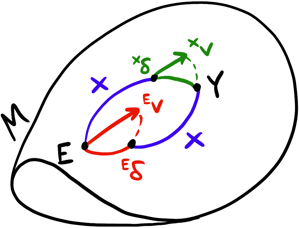
In the previous post, we ended with defining the global and local frames and the $\oplus$ and $\ominus$ operators. However, since we have these two global and local frames, how do we relate them? Note that these might be at different places in the manifold so we can’t simply use the $\Exp$ or $\Log$ operators directly. Unfortunately, we can’t continue without defining some reasonable axioms. So let’s go ahead and identify the left and right $\oplus$ operators.
\[X \oplus {}^Xv={}^Ev\oplus X\]Now let’s expand the $\oplus$ on both sides and simplify
\[\begin{align*} X \oplus {}^Xv & ={}^Ev\oplus X\\ \Exp({}^Ev^\wedge)X &= X~\Exp({}^Xv)\\ \exp({}^Ev^\wedge) &= X\exp({}^Xv^\wedge)X^{-1}=\exp(X{}^Xv^\wedge X^{-1})\\ {}^Ev^\wedge &= X{}^Xv^\wedge X^{-1} \end{align*}\]Note that in the third line we use a property of the exponential map that $X\exp({}^Xv^\wedge)X^{-1}=\exp(X{}^Xv^\wedge X^{-1})$. In the last line, notice that we relate the the tangent space $T_X M$ to the tangent space $T_E M$; in other words, we can bring a vector in the local frame to a vector in the global frame. This turns out to be a useful-enough operation that we give it a name: the adjoint:
\[\Ad_X : \mathfrak{m}\to\mathfrak{m}; v^\wedge\mapsto\Ad_Xv^\wedge\equiv X{}^Xv^\wedge X^{-1}\]The adjoint map sends vectors in the local frame to vectors in the global frame. Equivalently, we can say ${}^E v^\wedge=\Ad_X {}^X v^\wedge$. The adjoint at $X$ brings ${}^Xv^\wedge$ to ${}^Ev^\wedge$. Similar to the exponential map, this mapping is exact. From the definition, we can derive several properties:
- Linearity: $\Ad_X (av^\wedge+bw^\wedge) = a\Ad_X v^\wedge+b\Ad_X w^\wedge$
- Homomorphism: $\Ad_Y\Ad_Y v^\wedge=\Ad_{XY}v^\wedge$ We can also define an adjoint map more directly to map between two tangent spaces.
This map also has properties
- $X\oplus{}^Xv = (\Ad_X{}^Xv)\oplus X = {}^Ev\oplus X$
- $\Ad_{X^{-1} }=\Ad_X^{-1}$
- $\Ad_X\Ad_Y=\Ad_{XY}$

As a simple example, we can consider the set of rotations on the plane $SO(2)$. Since rotations on the plane communte everywhere, the mapping the left and right lead to the same result so the adjoint is just the identity: $\Ad_X=I = X\oplus {}^Xv={}^Ev\oplus X$ .
As a more complex example, consider $SO(3)$. We know rotations in space don’t commute, but if we compute the adjoint, we can figure out how exactly they commute (in other words, which term is missing). To do this, let’s pick an arbitrary $[\omega]_\times\in\mathfrak{so}(3)$ and $R\in SO(3)$. We’ll remove these later since they’re arbitrary anyways. Instead of starting immediately with the final definition, it’s a bit more illustrative to start a few steps above in the adjoint derivation.
\[R\exp([w]_\times) = \exp([\Ad_R~\omega]_\times)R\]On the left, we have a rotation matrix times another rotation matrix, but expressed in the Lie algebra $\omega$. In other words, we could have written $R’=\exp([w]_\times)$. But remember the adjoint operates in the Lie algebra (or corresponding vector space) so we need this extra decomposition. On the right side, we have commuted the two but applied the adjoint since it maps across vector spaces.
\[\begin{align*} R\exp([w]_\times) &= \exp([\Ad_R~\omega]_\times)R\\ \exp([\Ad_R~\omega]_\times)R &= R\exp([w]_\times)\\ \exp([\Ad_R~\omega]_\times) &= R\exp([w]_\times)R^{-1}\\ \exp([\Ad_R~\omega]_\times) &= \exp(R[w]_\times R^{-1})\\ [\Ad_R~\omega]_\times &= R [w]_\times R^{-1}\\ [\Ad_R~\omega]_\times &= [Rw]_\times\\ \Ad_R &= R\\ \end{align*}\]In the second-to-last step we use a property of the $[\cdot]_\times$ operator $R[\omega]_\times R^{-1}=[Rw]_\times$. Also, in the last step, we removed the $[\omega]_\times$ since it was arbitrary in the first place. So the adjoint of $SO(3)$ is the same as the rotation matrix $R$! This tells us how to relate commutations for 3D rotations.
Calculus on Lie Groups
Now we have all of the pieces to develop calculus on Lie Groups which we need to compute derivatives for optimization or any other kind of state estimation. The principle for calculus on Lie Groups is same as the original motivation: we want to avoid working directly on the manifold but rather in the tangent space. Tying this to state estimation, if we have a nonlinear motion model using Lie Groups, we need to compute Jacobians which means we need calculus on Lie Groups.
Recall for a scalar function $f:\R\to\R$ the definition of a derivative is
\[f'(x) = \lim_{h\to 0}\frac{f(x+h)-f(x)}{h}\]For a multivariate function $f:\R^n\to\R$, we can compute a gradient vector of partial derivatives:
\[\nabla f=\left[\frac{\p f}{\p x_1},\cdots,\frac{\p f}{\p x_n}\right]^T\]For a multivariate in-out function $f: \R^n\to\R^m$, can compute a Jacobian matrix of partial derivatives:
\[J = \frac{\p \vec{f} }{\p \vec{x} } = \begin{bmatrix} \frac{\p f_1}{\p x_1} & \cdots & \frac{\p f_1}{\p x_n}\\ \vdots & \ddots & \vdots\\ \frac{\p f_m}{\p x_1} & \cdots & \frac{\p f_m}{\p x_n} \end{bmatrix}\]Note that the intermediate notation I used $\frac{\p \vec{f} }{\p \vec{x} }$ is not well-defined but intended to be illustrative. Now suppose we have a function $f:G\to G$ on a Lie Group. We want to compute $\frac{\D f}{\D X}$. In other words, we want to know how a wiggle in $X\in G$ wiggles $f(X)\in G$. But what does it mean to wiggle $X$? This was well-defined for a scalar but not for a group element.
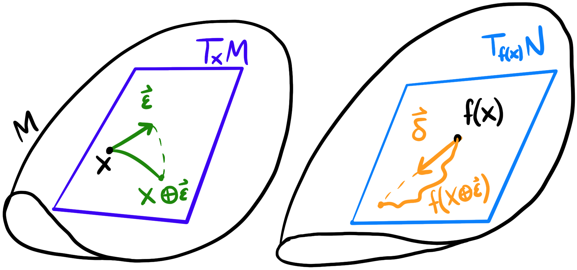
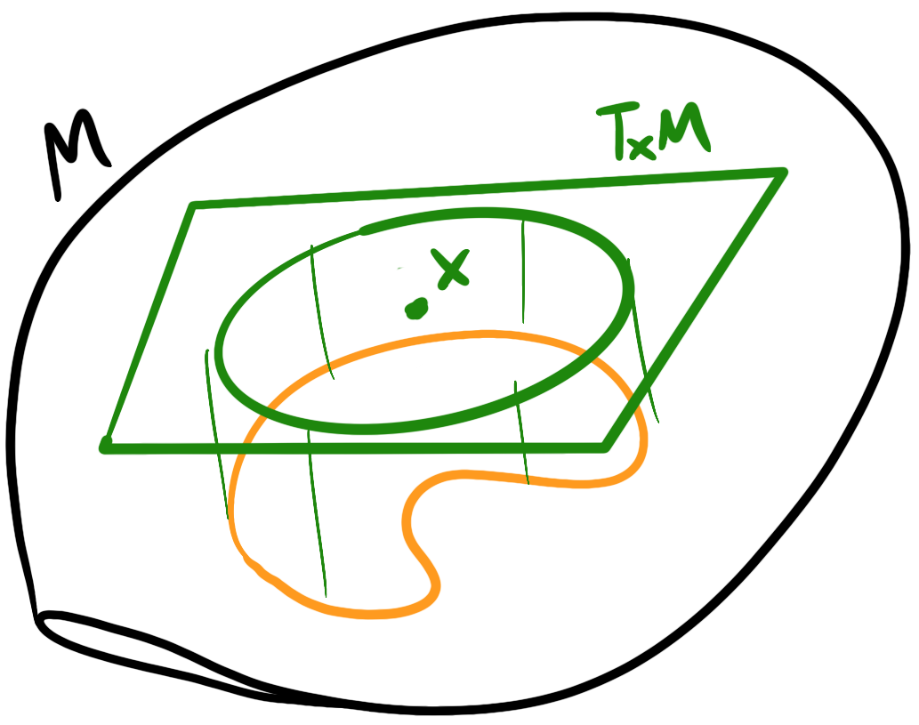
The key idea is that we use some small wiggle $\vec\varepsilon$ in the tangent space of $X$ rather than $X$ itself and map that wiggle to the manifold using the exponential map.

Notationally, we can write something like
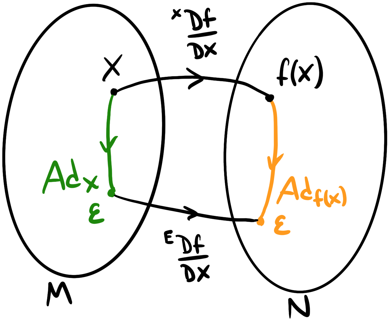
\[\begin{align*} \frac{ {}^X\D f}{\D X}&=\lim_{\vec\varepsilon\to 0}\frac{f(X\oplus\vec\varepsilon)\ominus f(X)}{\vec\varepsilon}\\ &=\lim_{\vec\varepsilon\to 0}\frac{\Log(f(X)^{-1}\circ f(X\cdot\Exp(\vec\varepsilon)))}{\vec\varepsilon}\\ &=\frac{\p}{\p\vec\varepsilon}\left[\Log(f(X)^{-1}\circ f(X\cdot\Exp(\vec\varepsilon)))\right]_{\vec\varepsilon=0}\\ \end{align*}\]Note that we had to “upgrade” $+$ to $\oplus$ and $-$ and $\ominus$ since we’re dealing with manifolds and tangent spaces. We’re being a bit sloppy with notation since vector division isn’t well-defined. If we want to be a bit more accurate, we should use $h\vec\varepsilon_i$ such that $h\in\R, \vert\vert h\vert\vert « 1$ where $\vec\varepsilon_i$ is a basis in the $i$ direction and and we take the limit with respect to $h$. Then we need to stack all of the $i$ bases.
\[\frac{ {}^X\D f}{\D X_i} =\lim_{h\to 0}\frac{f(X\oplus h\vec\varepsilon_i)\ominus f(X)}{\vec\varepsilon}\]Using that key idea, we’ve expressed variations in $X$ of $f(X)$ entirely in the tangent space. This Jacobian linearly maps tangent spaces $T_X M\cong\R^m\to T_{f(X)} M\cong\R^n$.
This new kind of derivative behaves similar to a normal derivative in that, for small variations:
\[f(X\oplus\vec\varepsilon)\approx f(X)\oplus\frac{\D f}{\D X}\vec\varepsilon\]To make the derivative more concrete, let’s try to compute the Jacobian of $SO(2)$ under the group action $Rv$, rotating a vector $v\in\R^2$ using a rotation matrix $R\in SO(2)$. Specifically, $f(R)=Rv$.
\[\begin{align*} \frac{ {}^R\D~ ~(Rv)}{\D R}&=\lim_{\theta\to 0}\frac{(R\oplus\theta)v\ominus Rv}{\theta}\\ &=\lim_{\theta\to 0}\frac{R~\Exp(\theta) v - Rv}{\theta}\\ &=\lim_{\theta\to 0}\frac{R(I + [\theta]_\times) v - Rv}{\theta}\\ &=\lim_{\theta\to 0}\frac{R[\theta]_\times v}{\theta}\\ &=\lim_{\theta\to 0}\frac{-R[1]_\times v~\theta}{\theta}\\ &=-R[1]_\times v\\ \end{align*}\]Note that since rotations in the plane commute $R\ominus S=\theta_R - \theta_S$ where $\theta\in\R$ is the corresponding angle to the 2D rotation matrix $R\in SO(2)$. We also expand the exponential map using a Taylor series $\Exp(\theta)\approx I +[\theta]_\times$ since the higher order terms vanish in the limit. We also use a useful property that $[a]_\times b= -a[b]_\times$. The other derivative is much simpler:
\[\frac{ {}^R\D~ ~(Rv)}{\D v}=R\]So far, we’ve been using the right $\oplus$ operator for now; this creates a mapping between local tangent spaces $T_X M\to T_{f(X)} N$. We could also define the left Jacobian $\frac{ {}^E\D f}{\D X}$ using the left $\oplus$ operator that creates a mapping between global tangent spaces $T_E M\to T_{E} N$. The maths is pretty straightforward to define, and we can relate the two using the adjoint.

So now we’re able to do calculus on Lie Groups by taking the derivative of a function with respect to a point on the manifold. Now for motion models, we can apply derivatives to compute the Jacobian of the motion model! Recall that for an on-manifold motion model, we take an initial pose $X_0$ and twists $v_i$ at some frequency $\Delta t_i$ and apply the exponential map iteratively:
\[\begin{align*} X_k&=X_0\oplus v_1\Delta t_1\oplus\cdots\oplus v_k\Delta t_k\\ &=X_0\Exp(v_1\Delta t_1)\cdots\Exp(v_k\Delta t_k)\\ \end{align*}\]The exponential map performs continuous integration on the manifold. However, with that motion model, we need to compute the derivative of the exponential map.
Jacobian Blocks
We’ll need some building blocks before computing things like the Jacobian of the exponential map and its inverse.
The first tool we’ll need is chain rule! This operates on Lie Groups exactly in the same way as ordinary calculus:
\[\frac{\D Z}{\D X} = \frac{\D Z}{\D Y}\frac{\D Y}{\D X}\]Next, we’ll need to prove the Jacobian of the inverse $f(X)=X^{-1}$ :
\[\begin{align*} \frac{\D X^{-1} }{\D X} &=\lim_{v\to 0}\frac{\Log[(X^{-1})^{-1}(X~\Exp(v))^{-1}]}{v}\\ &=\lim_{v\to 0}\frac{\Log(X~\Exp(v)^{-1}X^{-1})}{v}\\ &=\lim_{v\to 0}\frac{\Log(X~\Exp(-v)X^{-1})}{v}\\ &=\lim_{v\to 0}\frac{X~(-v)^{\wedge}X^{-1} }{v}\\ &=\lim_{v\to 0}\frac{\Ad_X(-v)}{v}\\ &=\lim_{v\to 0}\frac{-\Ad_X(v)}{v}\\ &=-\Ad_X\\ \end{align*}\]In the last step we removed $v$ since it was arbitrary. Now let’s prove composition $f(X,Y)=X\circ Y$ with respect to the first argument
\[\begin{align*} \frac{\D}{\D X}(X\circ Y) &=\lim_{v\to 0}\frac{\Log[f(X,Y)^{-1} f(X\Exp(v), Y)]}{v}\\ &=\lim_{v\to 0}\frac{\Log[(XY)^{-1} X~\Exp(v) Y]}{v}\\ &=\lim_{v\to 0}\frac{\Log[Y^{-1} X^{-1} X~\Exp(v) Y]}{v}\\ &=\lim_{v\to 0}\frac{\Log[Y^{-1} \Exp(v) Y]}{v}\\ &=\lim_{v\to 0}\frac{[Y^{-1}~\Exp(v) Y]^\vee}{v}\\ &=\lim_{v\to 0}\frac{\Ad_{Y^{-1} }v}{v}\\ &=\Ad_{Y^{-1} }\\ &=\Ad_Y^{-1}\\ \end{align*}\]and with respect to the second argument
\[\begin{align*} \frac{\D}{\D Y}(X\circ Y) &=\lim_{v\to 0}\frac{\Log[f(X,Y)^{-1}\circ f(X, Y~\Exp(v))]}{v}\\ &=\lim_{v\to 0}\frac{\Log[(X\circ Y)^{-1}\circ XY~\Exp(v)]}{v}\\ &=\lim_{v\to 0}\frac{\Log[(Y^{-1}X^{-1}\circ XY~\Exp(v)]}{v}\\ &=\lim_{v\to 0}\frac{\Log[\Exp(v)]}{v}\\ &=\frac{v}{v}\\ &= I \end{align*}\]Now that we have these blocks, we can define the right Jacobian as the derivative of the exponential map in the local frame.
\[J_r(v)=\frac{ {}^X\D}{\D v}\Exp(v)\]And the left Jacobian as the derivative of the exponential map in the global frame.
\[J_l(v)=\frac{ {}^E\D}{\D v}\Exp(v)\]Like other global and local frame relations, we can relate the two using the adjoint
\[\Ad_{\Exp(v)}=J_l(v)J_r^{-1}(v)\]This is where things get really complicated because, even for known manifolds, computing the closed forms for these Jacobians is super difficult so I’ll have to gloss over the details.
Now that we have some building blocks, we can compute Jacobians for the remaining operations like $\Log$, $\oplus$, and $\ominus$:
\[\begin{align*} \frac{\D}{\D X}\Log(X)&=J_r^{-1}(\Log(X))\\ \frac{\D}{\D X}(X\oplus v)&=\Ad_{\Exp(v)}^{-1} & \frac{\D}{\D X}(Y\ominus X)=-J_l^{-1}(Y\ominus X)\\ \frac{\D}{\D v}(X\oplus v)&=J_r(v) & \frac{\D}{\D Y}(Y\ominus X)=J_r^{-1}(Y\ominus X)\\ \end{align*}\]These can be proven using the chain rule we showed earlier.
Uncertainty on Manifolds
The last piece we’re missing is how to compute uncertainties on manifolds. Similar to a state estimate, uncertainty is also localized to the tangent space at some point (state estimate) $X$. We can define a mean $\bar{X}\in M$ and a perturbation $\sigma\in T_{\bar{X} } M$ in the tangent space at $\bar{X}$!

Then we can use $\ominus$ to compute uncertainties.
\[\begin{align*} X&=\bar{X}\oplus\sigma\\ \sigma &=X\ominus \bar{X} \end{align*}\]We can define a covariance in the local frame using the definition of covariance too:
\[{}^{X}\Sigma=\mathbb{E}[\sigma\sigma^T]=\mathbb{E}[(X\ominus \bar{X})(X\ominus \bar{X})^T]\]With this, we can define Gaussians on the manifold $\mathcal{N}(\bar{X},{}^{X}\Sigma)$. Note that the covariance is of the tangent perturbation.
Motion Integration using Lie Groups
Now we can get back to the question at hand: how do we perform motion integration on Lie Groups for things like EKFs. In the previous post we defined the motion model
\[\begin{align*} X_{i+1}&=X_i\oplus v=X_i\Exp(v)\\ P_{i+1}&=FP_{i}F^T+GW_iG^T \end{align*}\]where
- $X_i$ is the state at timestep $i$
- $v$ is the twist (linear and angular velocities)
- $P_i$ is the covariance at timestep $i$
- $F$ is the Jacobian of the motion model with respect to $X$
- $G$ is the Jacobian of the motion model with respect to $v$
- $W_i$ is the Gaussian noise matrix at timestep $i$
Now that we have the Jacobian blocks we can actually compute $F$ and $G$!
\[\begin{align*} F&=\frac{\D}{\D X}[X\oplus v] = \Ad_{\Exp(v)}^{-1}\\ G&=\frac{\D}{\D v}[X\oplus v] = J_r(v) \end{align*}\]With this, we have the full equations for state estimation on the manifold! Lie Groups don’t only work for EKFs though; we can apply the same logic to pose graph optimization or any other kind of optimization.
Conclusion
In this post, we wrapped up the discussion on Lie Groups by finishing on-manifold motion integration equations for state estimation. We started with defining the adjoint to relate the global and local frames. Then we took our familiar notion of calculus and extended it to work with Lie Groups. We also derived a few fundamental Jacobian blocks to use as a basis for more complicated derivatives. Using those blocks, we also were able to show how uncertainty propagates on a manifold. With all of that background, we were finally able to show the full equations of motion integration.
As I stated before, Lie Groups are pretty theoretical compared to other kinds of applied maths for engineering. Fortunately, there are libraries that abstract away the details of these implementations but it’s still important to know when Lie Groups might be useful. There’s still a lot more to Lie Groups but I’ve covered enough in these two posts for them to prove useful to you should you encounter a scenario where you’re on a manifold working with functions 🙂