Manifolds - Part 3
In the previous article, we constructed a manifold from just open sets and reinvented vectors, tangent spaces, dual vectors, cotangent spaces, and general tensors using the language of a manifold, i.e., without assuming flat coordinates. In this post, we’re going to discuss and derive the most important property of a manifold: curvature!
Covariant Derivatives
To discuss curvature, we’ll need some extra constructs. Curvature in a flat space involves taking second derivatives, but we haven’t actually discussed how to do calculus on manifolds. Partial derivatives and gradients only counted as basis vectors, not a calculus operations. But maybe they can do both. Let’s ask an important question about the partial derivative: does it transform like a tensor? If it does, we can simply use it as the primary method of doing calculus on manifolds. If not, then we need to invent some kind of derivative operator that does transform like a tensor. Let’s find out the answer by applying a coordinate transform to the partial derivative $\p_{\mu’}$ to a vector $V$:
\[\begin{align*} \frac{\p}{\p x^{\mu'}}V^{\nu'}&=\Big(\frac{\p x^\mu}{\p x^{\mu'}}\frac{\p}{\p x^\mu}\Big) \Big(\frac{\p x^{\nu'}}{\p x^{\nu}}V^\nu\Big)\\ &=\frac{\p x^\mu}{\p x^{\mu'}}\frac{\p}{\p x^\mu} \Big(\frac{\p x^{\nu'}}{\p x^{\nu}}V^\nu\Big)\\ &=\frac{\p x^\mu}{\p x^{\mu'}}\Big(\frac{\p x^{\nu'}}{\p x^\nu} \frac{\p}{\p x^{\mu}}V^\nu+V^\nu\frac{\p}{\p x^\mu}\frac{\p x^{\nu'}}{\p x^\nu}\Big)\\ &=\underbrace{\frac{\p x^\mu}{\p x^{\mu'}}\frac{\p x^{\nu'}}{\p x^\nu} \frac{\p}{\p x^{\mu}}V^\nu}_\text{transforms like a tensor}+\underbrace{V^\nu\frac{\p x^\mu}{\p x^{\mu'}}\frac{\p}{\p x^\mu}\frac{\p x^{\nu'}}{\p x^\nu}}_\text{doesn't transform like a tensor}\\ \end{align*}\](Note: going from the second to the third line, we used the product rule since $\frac{\p}{\p x^\mu}$ is a derivative operator.)
It doesn’t seem like partial derivatives transform like tensors! So it’s not a good derivative operator for us to do calculus on manifolds, unfortunately. We’ll have to invent our own derivative operator such that it produces a tensor when acting on vectors, duals, and tensors. What kind of properties do we want in a “good” derivative operator?
- Just like $\p_\mu$, we’d like to send $(k, l)$-rank tensors to $(k,l+1)$-rank tensors.
- Just like $\p_\mu$, we’d like to obey the Leibniz product rule (and thus linearity).
Since the partial derivative almost transforms like a tensor except for the non-tensorial part, we can use it as the base, but add a correction to account for the non-tensorial part. Actually, if we closely inspect the non-tensorial part, it seems to be taking the derivative of the basis; in other words, it accounts for the changing basis from point-to-point. We need a correction for each component so that means we need a linear transform for each. Therefore, the general form of the correction is a set of $n$ matrices $(\Gamma_\mu)^\nu_\lambda$. The outer upper and lower indices mean this is a linear transform, and the inner lower indicates we have $n$ of them.
We define the covariant derivative $\nabla$ as a generalization of the partial derivative but for arbitrary coordinates. We can think of it as the partial derivative with a correction for the changing basis. As it turns out (and that we’ll soon prove), the correction matrices $\Gamma^\nu_{\mu\lambda}$ do not transform like tensors so we don’t have to be so careful about the index placement because we can’t raise and lower indices on $\Gamma^\nu_{\mu\lambda}$ anyways. But in which basis does the correction happen? Well we might as well use the same basis used to define the vector we’re operating on; after all, it’s right there! With that, we can mathematically define the covariant derivative.
\[\nabla_\mu V^\nu\equiv\underbrace{\p_\mu V^\nu}_\text{partial}+\underbrace{\Gamma^\nu_{\mu\lambda}V^\lambda}_\text{correction}\]The correction matrices are special enough that we call them the connection coefficients or Christoffel symbols. Another way to think about this is that the covariant derivative tells us the change in $V^\nu$ in the $\mu$ direction. The complete geometric picture won’t make complete sense until we discuss parallel transport and geodesics soon, but I’ll present it here with some hand-waving.
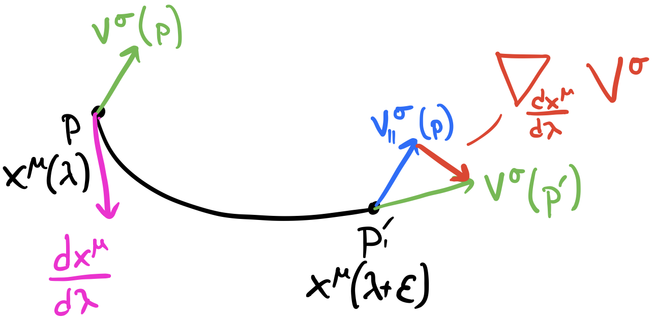
There are a few key actors to understanding the geometry of the covariant derivative. The first is having a vector $V$ at a point $p$. We have another point $q$ and a different value of $V$ at that point. Remember that vector fields are defined at each point on the manifold. The $\mu$ represents the tangent vector to some curve at $p$ that connects to $q$. If we were to take $V$ and move it along the curve in such a way to keep it “as straight as possible”, we’d end up with a different vector $V_{||}$ at $q$. The covariant derivative is just the difference between $V$ at $q$ and the “translated” vector $V_{||}$. Don’t worry if this doesn’t make perfect sense now; we’ll revisit this when we have a more rigourous definition of moving a vector “as straight as possible” along a curve.
The point to remember is that the connection coefficients are the correction matrices, i.e., the non-tensorial part.
\[\begin{align*} \Gamma^\nu_{\mu\lambda}&=\text{change in }\p_\mu\text{ caused by }\lambda\text{ in the }\p_\nu\text{ direction.}\\ &=\frac{\p^2 x^\nu}{\p x^\mu\p x^\lambda} \end{align*}\]I’ve said multiple times now that the connection coefficients represent the non-tensorial part so are they actually tensors? It turns out they are not. Let’s see why. First, let’s start with the above definition of the covariant derivative acting on a vector $V$.
\[\begin{align*} \nabla_\mu V^\nu &= \p_\mu V^\nu + \Gamma_{\mu\lambda}^\nu V^{\lambda}\\ \nabla_{\mu'} V^{\nu'} &= \p_{\mu'} V^{\nu'} + \Gamma_{\mu'\lambda'}^{\nu'} V^{\lambda'} \end{align*}\]Now we’re going to simply demand that the covariant derivative transform like a tensor.
\[\nabla_{\mu'} V^{\nu'} = \frac{\p x^\mu}{\p x^{\mu'}}\frac{\p x^{\nu'}}{\p x^\nu}\nabla_\mu V^\nu\]Since we’re inventing the covariant derivative for the sole purpose of being a tensorial operator on a manifold, demaning this constraint is a reasonable thing to do. Now we need to expand this equation to write the primed connection coefficients in terms of the unprimed ones. To start, let’s just consider the left-hand side and transform what we can transform from the primed to the unprimed coordinates.
\[\begin{align*} \nabla_{\mu'} V^{\nu'} &= \p_{\mu'} V^{\nu'} + \Gamma_{\mu'\lambda'}^{\nu'} V^{\lambda'}\\ &=\frac{\p x^\mu}{\p x^{\mu'}}\p_\mu\Big(\frac{\p x^{\nu'}}{\p x^\nu} V^\nu \Big) + \Gamma_{\mu'\lambda'}^{\nu'} \frac{\p x^{\lambda'}}{\p x^{\lambda}}V^{\lambda}\\ &=\frac{\p x^\mu}{\p x^{\mu'}}\frac{\p x^{\nu'}}{\p x^{\nu}}\p_\mu V^\nu + \frac{\p x^\mu}{\p x^{\mu'}}V^\nu\frac{\p}{\p x^\mu}\frac{\p x^{\nu'}}{\p x^{\nu}} + \Gamma_{\mu'\lambda'}^{\nu'}\frac{\p x^{\lambda'}}{\p x^{\lambda}}V^\lambda \end{align*}\]Just like we figured out the other tensor transformation rules, let’s expand the primed coordinates in terms of the unprimed ones using coordinate transforms. For the time being, let’s leave the connection coefficients untransformed since we don’t yet know how to transform them. Taking the above equation and adding back the right-hand side:
\[\require{cancel} \begin{align*} \nabla_{\mu'} V^{\nu'} &= \frac{\p x^\mu}{\p x^{\mu'}}\frac{\p x^{\nu'}}{\p x^\nu}\nabla_\mu V^\nu\\ \cancel{\frac{\p x^\mu}{\p x^{\mu'}}\frac{\p x^{\nu'}}{\p x^{\nu}}\p_\mu V^\nu} + \frac{\p x^\mu}{\p x^{\mu'}}V^\nu\frac{\p}{\p x^\mu}\frac{\p x^{\nu'}}{\p x^{\nu}} + \Gamma_{\mu'\lambda'}^{\nu'}\frac{\p x^{\lambda'}}{\p x^{\lambda}}V^\lambda &= \frac{\p x^\mu}{\p x^{\mu'}}\frac{\p x^{\nu'}}{\p x^\nu}(\cancel{\p_\mu V^\nu} + \Gamma_{\mu\lambda}^\nu V^{\lambda})\\ \frac{\p x^\mu}{\p x^{\mu'}}V^\nu\frac{\p}{\p x^\mu}\frac{\p x^{\nu'}}{\p x^{\nu}} + \Gamma_{\mu'\lambda'}^{\nu'}\frac{\p x^{\lambda'}}{\p x^{\lambda}}V^\lambda &= \frac{\p x^\mu}{\p x^{\mu'}}\frac{\p x^{\nu'}}{\p x^\nu}\Gamma_{\mu\lambda}^\nu V^{\lambda} \end{align*}\]We want to remove $V$ since it was arbitrary from the start, but we can’t since the indices don’t match up. We can make them match by relabeling $\nu$ to $\lambda$; this is completely legal since $\nu$ in $V^\nu$ and $\lambda$ in $V^\lambda$ are both dummy indices that we can relabel to anything convenient so let’s relabel everything to be $\lambda$ and get rid of $V$ entirely (and move the primed connection coefficients to one side of the equation and use second-order derivatives).
\[\begin{align*} \frac{\p x^\mu}{\p x^{\mu'}}V^\lambda\frac{\p}{\p x^\mu}\frac{\p x^{\nu'}}{\p x^{\lambda}} + \Gamma_{\mu'\lambda'}^{\nu'}\frac{\p x^{\lambda'}}{\p x^{\lambda}}V^\lambda &= \frac{\p x^\mu}{\p x^{\mu'}}\frac{\p x^{\nu'}}{\p x^\nu}\Gamma_{\mu\lambda}^\nu V^{\lambda}\\ \frac{\p x^\mu}{\p x^{\mu'}}\frac{\p}{\p x^\mu}\frac{\p x^{\nu'}}{\p x^{\lambda}} + \Gamma_{\mu'\lambda'}^{\nu'}\frac{\p x^{\lambda'}}{\p x^{\lambda}} &= \frac{\p x^\mu}{\p x^{\mu'}}\frac{\p x^{\nu'}}{\p x^\nu}\Gamma_{\mu\lambda}^\nu\\ \frac{\p x^{\lambda'}}{\p x^{\lambda}} \Gamma_{\mu'\lambda'}^{\nu'}&= \frac{\p x^\mu}{\p x^{\mu'}}\frac{\p x^{\nu'}}{\p x^\nu}\Gamma_{\mu\lambda}^\nu - \frac{\p x^\mu}{\p x^{\mu'}}\frac{\p}{\p x^\mu}\frac{\p x^{\nu'}}{\p x^{\lambda}}\\ \frac{\p x^{\lambda'}}{\p x^{\lambda}} \Gamma_{\mu'\lambda'}^{\nu'}&= \frac{\p x^\mu}{\p x^{\mu'}}\frac{\p x^{\nu'}}{\p x^\nu}\Gamma_{\mu\lambda}^\nu - \frac{\p x^\mu}{\p x^{\mu'}}\frac{\p^2 x^{\nu'}}{\p x^\mu\p x^{\lambda}} \end{align*}\]We’re almost done isolating the primed coordinates in terms of the unprimed coordinates, but we need to get rid of the leading $\frac{\p x^{\lambda’}}{\p x^\lambda}$ on the left-hand side. A convenient strategy for removing terms of this form is to exploit the property of the Kronecker delta: $\frac{\p x^{\lambda}}{\p x^{\rho’}}\frac{\p x^{\lambda’}}{\p x^{\lambda}}=\delta_{\rho’}^{\lambda’}$. So we can multiply both sides by $\frac{\p x^{\lambda}}{\p x^{\rho’}}$ and get a Kronecker delta on the left-hand side that we can replace by swapping indices:
\[\begin{align*} \frac{\p x^{\lambda}}{\p x^{\rho'}}\frac{\p x^{\lambda'}}{\p x^{\lambda}} \Gamma_{\mu'\lambda'}^{\nu'}&= \frac{\p x^{\lambda}}{\p x^{\rho'}}\frac{\p x^\mu}{\p x^{\mu'}}\frac{\p x^{\nu'}}{\p x^\nu}\Gamma_{\mu\lambda}^\nu - \frac{\p x^{\lambda}}{\p x^{\rho'}}\frac{\p x^\mu}{\p x^{\mu'}}\frac{\p^2 x^{\nu'}}{\p x^\mu\p x^{\lambda}}\\ \delta_{\rho'}^{\lambda'} \Gamma_{\mu'\lambda'}^{\nu'}&= \frac{\p x^{\lambda}}{\p x^{\rho'}}\frac{\p x^\mu}{\p x^{\mu'}}\frac{\p x^{\nu'}}{\p x^\nu}\Gamma_{\mu\lambda}^\nu - \frac{\p x^{\lambda}}{\p x^{\rho'}}\frac{\p x^\mu}{\p x^{\mu'}}\frac{\p^2 x^{\nu'}}{\p x^\mu\p x^{\lambda}}\\ \Gamma_{\mu'\rho'}^{\nu'}&= \frac{\p x^{\lambda}}{\p x^{\rho'}}\frac{\p x^\mu}{\p x^{\mu'}}\frac{\p x^{\nu'}}{\p x^\nu}\Gamma_{\mu\lambda}^\nu - \frac{\p x^{\lambda}}{\p x^{\rho'}}\frac{\p x^\mu}{\p x^{\mu'}}\frac{\p^2 x^{\nu'}}{\p x^\mu\p x^{\lambda}}\\ \end{align*}\]Now we can finally relabel $\rho’$ to $\lambda’$ to be more consistent with the original notation. This is also legal to do since $\rho’$ is also a dummy index that we’re free to relabel.
\[\Gamma_{\mu'\lambda'}^{\nu'} = \underbrace{\frac{\p x^{\lambda}}{\p x^{\lambda'}}\frac{\p x^\mu}{\p x^{\mu'}}\frac{\p x^{\nu'}}{\p x^\nu}\Gamma_{\mu\lambda}^\nu}_{\text{tensorial-like}} - \underbrace{\frac{\p x^{\lambda}}{\p x^{\lambda'}}\frac{\p x^\mu}{\p x^{\mu'}}\frac{\p^2 x^{\nu'}}{\p x^\mu\p x^{\lambda}}}_{\text{non-tensorial-like}}\]From this equation, we see that the first term seems to look like a valid transform; however, the second term is some second-order quantity that ruins the ability for the connection coefficients to transform like tensors. If that second term was zero, then we could say the connection coefficients transform like a tensor, but, from its existence, we can say that the connection coefficients do not transform like tensors. In fact, we can even say that the connection coefficients are intentionally non-tensorial to cancel the non-tensorial part of the partial derivative that we saw earlier. The consequence of non-tensorial terms means we can’t raise or lower indices on the connection coefficients with the metric tensor, but it also means we can be more haphazard with the index placement and leave one upper and two lower indices 😉
So far, we’ve shown the action of the covariant derivative on vectors, but what about its action on covectors? If we can figure out how to apply it to both vectors and covectors, we can generalize its action on arbitrary tensors. Similar to what we did with vectors, we can simply demand that the result of the covariant derivative transforms like a tensor.
\[\nabla_\mu\omega_\nu = \p_\mu\omega_\nu + \Theta_{\mu\nu}^\lambda\omega_\lambda\]We’re using $\Theta$ because, at this point in time, we have no reason to believe that $\Theta$ and $\Gamma$ are related. Spoiler alert: they are! In order to operate the covariant derivative on covectors, we need to impose/demand two more constraints:
- It commutes with contractions: $\nabla_\mu (T_{\nu\lambda}^{\lambda})=(\nabla T)_{\mu\nu\lambda}^\lambda$
- It reduces to the partial derivative on scalar (functions) $\phi$: $\nabla_\mu \phi = \p_\mu\phi$
Like last time, we can apply a covector to a vector to get a scalar.
\[\begin{align*} \nabla_\mu(\omega_\lambda V^\lambda) &= (\nabla_\mu\omega_\lambda)V^\lambda + \omega_\lambda(\nabla_\mu V^\lambda)\\ &= (\p_\mu\omega_\lambda + \Theta_{\mu\lambda}^\sigma\omega_\sigma)V^\lambda + \omega_\lambda(\p_\mu V^\lambda+\Gamma_{\mu\rho}^\lambda V^\rho)\\ &= \p_\mu\omega_\lambda V^\lambda + \Theta_{\mu\lambda}^\sigma\omega_\sigma V^\lambda + \omega_\lambda\p_\mu V^\lambda+ \omega_\lambda\Gamma_{\mu\rho}^\lambda V^\rho\\ \end{align*}\]From the second constraint on the covariant derivative, we know that the left-hand side of the above equation reduces to the partial derivative acting on a scalar.
\[\begin{align*} \nabla_\mu(\omega_\lambda V^\lambda) &= \p_\mu(\omega_\lambda V^\lambda)\\ &= \p_\mu\omega_\lambda V^\lambda + \omega_\lambda\p_\mu V^\lambda \end{align*}\]Now let’s set both sides of the equation equal to each other to cancel out terms (and isolate $\Theta$).
\[\begin{align*} \cancel{\p_\mu\omega_\lambda V^\lambda} + \Theta_{\mu\lambda}^\sigma\omega_\sigma V^\lambda + \bcancel{\omega_\lambda\p_\mu V^\lambda} + \omega_\lambda\Gamma_{\mu\rho}^\lambda V^\rho &= \cancel{\p_\mu\omega_\lambda V^\lambda} + \bcancel{\omega_\lambda\p_\mu V^\lambda}\\ \Theta_{\mu\lambda}^\sigma\omega_\sigma V^\lambda + \omega_\lambda\Gamma_{\mu\rho}^\lambda V^\rho &= 0\\ \Theta_{\mu\lambda}^\sigma\omega_\sigma V^\lambda &= -\omega_\lambda\Gamma_{\mu\rho}^\lambda V^\rho\\ \end{align*}\](I’ve used two different kinds of slashes to note which of the like terms cancel.) To relate $\Theta$ and $\Gamma$, we need to get rid of $\omega$ and $V$. We can relabel them on the right-hand side by mapping $\lambda$ to $\sigma$ and $\rho$ to $\lambda$.
\[\Theta_{\mu\lambda}^\sigma\omega_\sigma V^\lambda = -\omega_\sigma\Gamma_{\mu\lambda}^\sigma V^\lambda\\\]Now we can remove $\omega$ and $V$.
\[\Theta_{\mu\lambda}^\sigma = -\Gamma_{\mu\lambda}^\sigma\\\]So $\Theta$ and $\Gamma$ are related by a negation! So we can make that substitution in the equation that applies the covariant derivative to covectors.
\[\nabla_\mu\omega_\nu \equiv \p_\mu\omega_\nu - \Gamma_{\mu\nu}^\lambda\omega_\lambda\]Take a second to compare the indices on the action of the covariant derivative on vectors versus covectors. For vectors, we have a positive connection coefficient whose second lower index becomes a dummy index across the vector’s index. For covectors, we have a negative connection coefficient whose only upper index becomes a dummy index across the covector’s index. With this observation, we can generalize to arbitrary tensors.
\[\begin{align*} \nabla_\lambda T_{\nu_1\cdots\nu_l}^{\mu_1\cdots\mu_k} &= \p_\lambda T_{\nu_1\cdots\nu_l}^{\mu_1\cdots\mu_k}\\ &+ \Gamma_{\lambda\sigma}^{\mu_1}T_{\nu_1\cdots\nu_l}^{\sigma\mu_2\cdots\mu_k}+\Gamma_{\lambda\sigma}^{\mu_2}T_{\nu_1\cdots\nu_l}^{\mu_1\sigma\cdots\mu_k}+\cdots+\Gamma_{\lambda\sigma}^{\mu_k}T_{\nu_1\cdots\nu_l}^{\mu_1\cdots\mu_{k-1}\sigma}\\ &- \Gamma_{\lambda\nu_1}^{\sigma}T_{\sigma\nu_2\cdots\nu_l}^{\mu_1\cdots\mu_k}-\Gamma_{\lambda\nu_2}^{\sigma}T_{\nu_1\sigma\cdots\nu_l}^{\mu_1\cdots\mu_k}-\cdots-\Gamma_{\lambda\nu_l}^{\sigma}T_{\nu_1\cdots\nu_{l-1}\sigma}^{\mu_1\cdots\mu_{k}}\\ \end{align*}\]There’s a pattern here depending on how many upper and lower indices. Take a second to understand the pattern since it’ll be useful later.
To quickly recap, we’ve successfully defined the covariant derivative on arbitrary tenors. However, in each definition, we write the covariant derivative in terms of the connection coefficients which, as a consequence of their non-tensorial-ness, are coordinate-dependent. We could use many different coordinates, which means we could have many different definitions of the covariant derivative! This is a fundamental characteristic of the covariant derivative and the connection coefficients, but we can define a unique connection if we impose some additional constraints: torsion-free and metric compatibility.
For a connection to be torsion-free, it must be symmetric in its lower indices.
\[\Gamma_{\mu\nu}^\lambda=\Gamma_{\nu\mu}^\lambda\]The consequence of a connection being torsion-free means, given a connection $\Gamma_{\mu\nu}^\lambda$, we can immediately define another connection with permutated lower indices $\Gamma_{\nu\mu}^\lambda$. In fact, we define the torsion tensor as $T_{\mu\nu}^\lambda = \Gamma_{\mu\nu}^\lambda - \Gamma_{\nu\mu}^\lambda = 2\Gamma_{[\mu\nu]}^\lambda$. Interestingly, the torsion tensor is a valid tensor, even though it is composed of the non-tensorial connection. To see this, suppose we had two connections $\nabla$ and $\tilde{\nabla}$. Let’s apply both on an arbitrary vector $V^\lambda$ and take the difference.
\[\begin{align*} \nabla_\mu V^\lambda-\tilde{\nabla}_\mu V^\lambda &= \cancel{\p_\mu V^\lambda} + \Gamma_{\mu\nu}^\lambda V^\nu - \cancel{\p_\mu V^\lambda} - \tilde{\Gamma}_{\mu\nu}^\lambda V^\nu\\ &= (\Gamma_{\mu\nu}^\lambda - \tilde{\Gamma}_{\mu\nu}^\lambda) V^\nu\\ &= S_{\mu\nu}^\lambda V^\nu\\ \end{align*}\]Since the left-hand side is a tensor, the right-hand side must also be a tensor, which means $S_{\mu\nu}^\lambda$, which is the difference of the connections, is also a tensor. Torsion is a special case of $S_{\mu\nu}^\lambda$ where we use the connection.

Geometrically, we can think of torsion as the “twisting” of reference frames or a “corkscrew” of reference frames along a path. We’ll get a slightly better geometric interpretation after we discuss parallel transport soon.
The second constraint we enforce is metric compatibility, which says $\nabla_\rho g_{\mu\nu}=0$. In words, that means the metric is flat/Euclidean at each individual point in the space. We need this property so that the covariant derivative commutes with the metric tensor when raising and lowering indices: $g_{\mu\lambda}\nabla_\rho V^\lambda = \nabla_\rho V_\mu$. Like with the covariant derivative action on covectors, there’s no way to prove these two constraints; we simply demand that they be true.
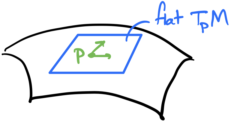
Metric compatibility means that components of the metric are constant at a point. Geometrically, this means, at a point, we can define a flat tangent space. Or, to be more precise, we can write the metric components in a way that they are constant.
Now that we have those two contraints, we can construct a unique connection from the metric using those two properties. Let’s first apply the covariant derivative to the metric tensor and set it to zero (using metric compatibility). With that one equation, we can can permute the indices to get two more equations.
\[\begin{align*} \nabla_\rho g_{\mu\nu} &= \p_\rho g_{\mu\nu} - \Gamma_{\rho\mu}^\lambda g_{\lambda\nu} - \Gamma_{\rho\nu}^\lambda g_{\mu\lambda} &= 0\\ \nabla_\mu g_{\nu\rho} &= \p_\mu g_{\nu\rho} - \Gamma_{\mu\nu}^\lambda g_{\lambda\rho} - \Gamma_{\mu\rho}^\lambda g_{\nu\lambda} &= 0\\ \nabla_\nu g_{\rho\mu} &= \p_\nu g_{\rho\mu} - \Gamma_{\nu\rho}^\lambda g_{\lambda\mu} - \Gamma_{\nu\mu}^\lambda g_{\rho\lambda} &= 0\\ \end{align*}\]Now we take the first equation and subtract the second and third equations. Then we can use the torsion-free property to cancel multiple terms, i.e., any connection coefficients with permuted lower indices.
\[\require{cancel} \begin{align*} \nabla_\rho g_{\mu\nu} &= \p_\rho g_{\mu\nu} - \cancel{\Gamma_{\rho\mu}^\lambda g_{\lambda\nu}} - \bcancel{\Gamma_{\rho\nu}^\lambda g_{\mu\lambda}} &= 0\\ -\nabla_\mu g_{\nu\rho} &= \p_\mu g_{\nu\rho} - \Gamma_{\mu\nu}^\lambda g_{\lambda\rho} - \cancel{\Gamma_{\mu\rho}^\lambda g_{\nu\lambda}} &= 0\\ -\nabla_\nu g_{\rho\mu} &= \p_\nu g_{\rho\mu} - \bcancel{\Gamma_{\nu\rho}^\lambda g_{\lambda\mu}} - \Gamma_{\nu\mu}^\lambda g_{\rho\lambda} &= 0\\ \end{align*}\]And we’re left with an equation with a single connection coefficient after permuting the indices so they match.
\[\begin{align*} \p_\rho g_{\mu\nu} - \p_\mu g_{\nu\rho} - \p_\nu g_{\rho\mu} + 2\Gamma_{\mu\nu}^\lambda g_{\lambda\rho} &= 0\\ \Gamma_{\mu\nu}^\lambda g_{\lambda\rho} &= \frac{1}{2}(\p_\mu g_{\nu\rho} + \p_\nu g_{\rho\mu} - \p_\rho g_{\mu\nu})\\ \end{align*}\]To get rid of the extra $g_{\lambda\rho}$, we can multiply by $g^{\sigma\rho}$ and use the Kronecker delta.
\[\begin{align*} \Gamma_{\mu\nu}^\lambda g_{\lambda\rho}g^{\sigma\rho} &= \frac{1}{2}g^{\sigma\rho}(\p_\mu g_{\nu\rho} + \p_\nu g_{\rho\mu} - \p_\rho g_{\mu\nu})\\ \Gamma_{\mu\nu}^\lambda \delta_{\lambda}^{\sigma} &= \frac{1}{2}g^{\sigma\rho}(\p_\mu g_{\nu\rho} + \p_\nu g_{\rho\mu} - \p_\rho g_{\mu\nu})\\ \Gamma_{\mu\nu}^\sigma &= \frac{1}{2}g^{\sigma\rho}(\p_\mu g_{\nu\rho} + \p_\nu g_{\rho\mu} - \p_\rho g_{\mu\nu})\\ \end{align*}\]Finally we’ve written the connection coefficients in terms of the metric! This unique connection is called the Christoffel/Levi-Civita/Riemannian connection. This is the canonical connection that’s used often in general relativity and other fields so we have a “preferred” covariant derivative. It’s not necessary to use this particular connection, especially if there is another set of connection coefficients that makes the particular problem we’re studying easier, but this connection is often used because it’s convenient.
Parallel Transport
Now that we have a clear definition of a “preferred” covariant derivative, we can do calculus on a manifold like we could in a flat space! However, we quickly run into a problem: how do we compare vectors on a manifold? With scalars, we can compare two of them at different points on a manifold, but we can’t compare two different vectors at two different points on the manifold since they would be in different tangent spaces! The vector might actually be the same in one tangent space but look different in the other tangent space (but still related by a transform).
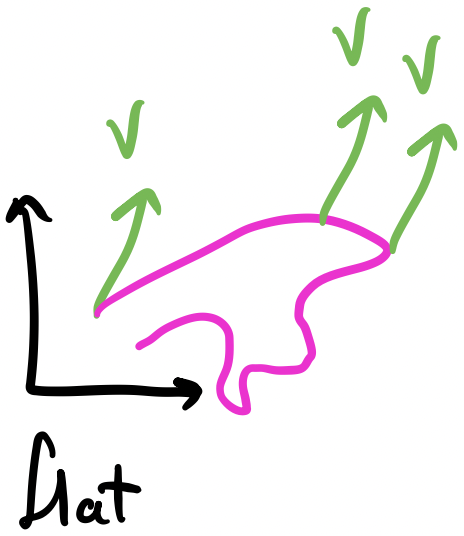
In a Cartesian space, if we have a vector $V$ and we move it along a path, it will forever have the same magnitude and direction. Some people say that vectors (in a Cartesian space) are just displacements that you can slide around the space because the displacement is relative: it doesn’t depend on where the arrow starts/ends. However, this is not true for curved coordinates.
In a flat space, we didn’t have to be this careful since we can arbitrary move a vector from point to point while keeping it parallel with itself. If we took a vector and drew an arbitrary path for the vector to take, at each point along the path, the vector would be pointed in exactly the same direction with the same magnitude! A consequence of this is that it doesn’t matter what the path, e.g., a long path and short path that have the same endpoint will still keep the vector the exact same.
Since it seems to work in flat space, let’s try this idea on a manifold: take a vector in one tangent space and “transport” it to the other tangent space so that the two vectors are in the same tangent space while keeping the “transported” vector “as straight as possible”. This notion is called parallel transport. We have to say “as straight as possible” since, in a curved space, it’s not always possible to keep a vector pointed completely in the same direction with the same magnitude at each point along the path. In fact, it’s even worse than that because the path we take will change the resulting vector!
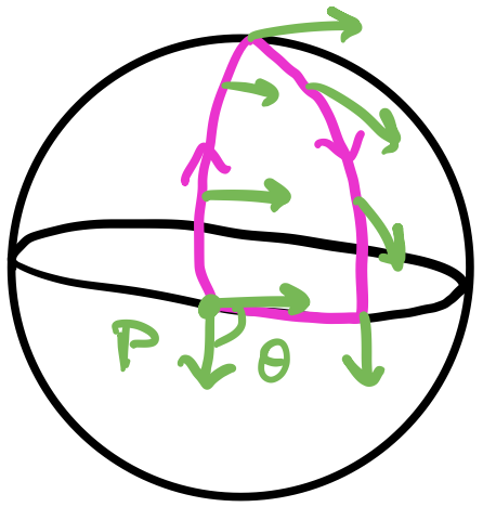
On a sphere, suppose we start at the equator with a vector pointing along the equator. Then we parallel transport that vector to the North Pole. Then we parallel transport it back to the equator on a different longitude. Finally, we parallel transport it along the equator back to its original position. We’ll find that it has rotated! It’s different from the original vector.
Even keeping the vector as straight as possible, the resulting vectors are pointed in completely different directions. Unfortunately, this is a fundamental fact about manifolds that we can’t get over with a clever trick or coordinate transform! But we can try to precisely define parallel transport and what we mean by “keeping the vector as straight as possible”. Mathematically, this means we want to keep the tensor components from changing as much as possible along the curve. Suppose we have a curve $x^\mu(\lambda)$ and an arbitrary tensor $T_{\nu_1\cdots\nu_l}^{\mu_1\cdots\mu_k}$. Then keeping the components the same just means the derivative of the tensor along the path must vanish.
\[\frac{\d}{\d\lambda}T_{\nu_1\cdots\nu_l}^{\mu_1\cdots\mu_k} = \frac{\d x^\sigma}{\d\lambda}\p_\sigma T_{\nu_1\cdots\nu_l}^{\mu_1\cdots\mu_k} = 0\]However this isn’t quite tensorial because we have a partial derivative. We can make this tensorial by replacing the partial derivative with a covariant derivative (this is sometimes called the “comma goes to semicolon” rule if you denote partials with commas and covariant derivatives with semicolons, but I hate that notation), and we get the equation of parallel transport.
\[\frac{\d x^\sigma}{\d\lambda}\nabla_\sigma T_{\nu_1\cdots\nu_l}^{\mu_1\cdots\mu_k} = 0\]For convenience, we can define a parallel transport operator/directional covariant derivative using the covariant derivative and a tangent vector.
\[\frac{\D}{\d\lambda} = \frac{\d x^\sigma}{\d\lambda}\nabla_\sigma\]Going back to our original inquiry, let’s see what this equation looks like for a vector $V^\mu$.
\[\begin{align*} \frac{\d x^\sigma}{\d\lambda}\nabla_\sigma V^\mu &= 0\\ \frac{\d x^\sigma}{\d\lambda}(\p_\sigma V^\mu + \Gamma_{\sigma\rho}^\mu V^\rho) &= 0\\ \frac{\d x^\sigma}{\d\lambda}\Big(\frac{\p}{\p x^\sigma} V^\mu + \Gamma_{\sigma\rho}^\mu V^\rho\Big) &= 0\\ \frac{\d}{\d\lambda} V^\mu + \Gamma_{\sigma\rho}^\mu \frac{\d x^\sigma}{\d\lambda} V^\rho &= 0\\ \end{align*}\]Note that this is a set of 1st order differential equations, one for each $\mu$ index. Also note that since the parallel transport equation depends on coordinate-dependent things like $\Gamma$ and $\frac{\d x^\sigma}{\d\lambda}$, the equation itself also depends on coordinates.
One immediately practical application of the parallel transport equation is to see what happens when we parallel transport the metric $g_{\mu\nu}$.
\[\require{cancel} \frac{\D}{\d\lambda}g_{\mu\nu} = \frac{\d x^\sigma}{\d\lambda}\cancelto{0}{\nabla_\sigma g_{\mu\nu}} = 0\]We can see that the metric is always parallel transported because of metric compatibility! This means that the value of inner products is preserved as we parallel transport along a curve.
Now suppose we also parallel transport two vectors that the metric acts on $V^\mu$ and $W^\nu$ along with it. Suppose those vectors are also parallel transported along with the metric.
\[\require{cancel} \begin{align*} \frac{\D}{\d\lambda}(g_{\mu\nu}V^\mu W^\nu) &= 0\\ \cancelto{0}{(\frac{\D}{\d\lambda}g_{\mu\nu})}V^\mu W^\nu + g_{\mu\nu}\cancelto{0}{(\frac{\D}{\d\lambda}V^\mu)} W^\nu + g_{\mu\nu}V^\mu\cancelto{0}{(\frac{\D}{\d\lambda}W^\nu)} &= 0 \end{align*}\]The first term is cancelled because of metric compatibility and the second and third terms are also cancelled because we defined $V^\mu$ and $W^\nu$ to be parallel transported. This means that norms, angles, and orthogonality are also preserved!
Now that we’ve discussed parallel transport, let me circle back to a few points geometrically and suppliment the lines and lines of equations with actual geometrical pictures. Let’s start with the geometrical picture of the covariant derivative. Recall that it generalizes the partial derivative by adding a correction for the changing basis that occurs from point-to-point. But, if a vector was parallel transported, by the parallel transport equation, the change in the covariant derivative along the path is zero. So we can think of the covariant derivative as being the vector that is the difference between parallel transporting a vector on a path from one point to another and simply evaluating the vector at that point on the manifold (see the first image in this post).
Additionally, with parallel transport, we can also get a slightly better geometric picture of torsion.
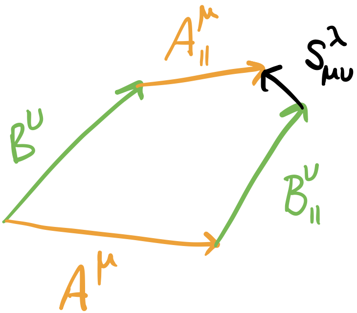
Suppose we have two vector fields $A^\mu$ and $B^\nu$. If we parallel transport $A^\mu$ in the direction of $B^\nu$ and $B^\nu$ in the direction of $A^\mu$, then the torsion tensor $S_{\mu\nu}^\lambda$ measures the ability of that loop to close. With a torsion-free metric, the parallel-transported vectors form a closed parallelogram.
Geodesics
One last crucial topic we’ll need to discuss before getting into curvature is a geodesic. To understand the intuition, remember that parallel transport changes a vector along a particular path from point to point. But there are an infinite number of paths between any two points so there doesn’t immediately seem to be a way to have a “preferred” path between two points that multiple people could compare. One candidate is picking the “shortest possible” path between the points. In a flat space, we knew how to do this: pick a straight line! But on a curved manifold where the coordinates change as well, there isn’t always a “straight” path.
One way to do this is to find a path $\frac{\d x^\mu}{\d\lambda}$ that minimizes the total arc length/path length between any two points. But this way requires us to know and use calculus of variations so that’s complicated! A slightly less formal, but more intuitive, way to understand a path length is in terms of parallel transport. One observation is that, in a flat space, a straight line keeps its tangent vector pointing in the same direction along the line. In other words, the straight line parallel transports its own tangent vector. This intuition carries over to a curved space. Suppose we have a curve $x^\mu(\lambda)$ and its tangent vector $\frac{\d x^\mu}{\d\lambda}$. Let’s parallel transport the tangent vector along the curve.
\[\begin{align*} \frac{\D}{\d\lambda}\Big(\frac{\d x^\mu}{\d\lambda}\Big) &= 0\\ \frac{\d x^\sigma}{\d\lambda}\nabla_\sigma\frac{\d x^\mu}{\d\lambda} &= 0\\ \frac{\d x^\sigma}{\d\lambda}\Big(\frac{\p}{\p x^\sigma}\frac{\d x^\mu}{\d\lambda} + \Gamma_{\sigma\rho}^\mu\frac{\d x^\rho}{\d\lambda}\Big) &= 0\\ \frac{\d}{\d\lambda}\frac{\d x^\mu}{\d\lambda} + \Gamma_{\sigma\rho}^\mu\frac{\d x^\sigma}{\d\lambda}\frac{\d x^\rho}{\d\lambda} &= 0\\ \frac{\d^2 x^\mu}{\d\lambda^2} + \Gamma_{\sigma\rho}^\mu\frac{\d x^\sigma}{\d\lambda}\frac{\d x^\rho}{\d\lambda} &= 0\\ \end{align*}\]The final result is the geodesic equation, a 2nd order differential equation, one for each coordinate/index $\mu$. Notice that in a Cartesian space, all $\Gamma=0$ so we’re left with $\frac{\d^2 x^\mu}{\d\lambda^2} = 0$. The solution to this differential equation is a line! (If you don’t know any differential equations, you can convince yourself of this since the only kinds of functions with no second derivative anywhere are lines!) Even without talking about curvature, geodesics are incredibly important: in general relativity, test particles in a gravitational field move along geodesics so they’re critical for understanding the consequences of different gravities.
Solving the geodesic equation can seem a little complicated so there’s an alternative way to think about geodesics that’s a bit more practical. Imagine we’re at an arbitrary point $p$ on a manifold, and we have a tangent vector $V^\mu$ to some curve/direction we want to travel in. We can construct a unique geodesic in a small neighborhood of $p$. Suppose our geodesic is $\gamma^\mu(\lambda)$. From the above statements, we immediately have two constraints to the geodesic: $\gamma^\mu(\lambda=0)=p$ and $\frac{\d\gamma^\mu}{\d\lambda}(\lambda=0)=V^\mu$. The former says that the geodesic “starts” at $p$ and the second statement says that the tangent vector at $\lambda=0$ on the geodesic is $V^\mu$. The exponential map is the map we use to get the geodesic. It is defined as $\exp_p: T_p\to M, V^\mu\mapsto\gamma^\mu(\lambda=1)$ such that $\gamma^\mu$ solves the geodesic equation.
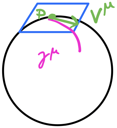
Given a point $p$ and a direction $V^\mu$ at $p$, it’s always possible to specify a unique geodesic $\gamma^\mu$ “in the neighborhood” of the point. If we stray too far from the point, this geodesic fails to be unique because they could cross over each other.
Since the geodesic is on the manifold, if we follow $\gamma^\mu$, then there’s some other point $q$ also on the manifold such that $\gamma^\mu(\lambda=1)=q$. After this process, we’re now at another point on the manifold by travelling along the geodesic. With this technique, we can travel all across the manifold by travelling from tangent space to tangent space along the shortest path. An important thing to note is that this geodesic is only unique and invertible in a “small enough” neighborhood around $p$. Travel too far away, and the we no longer have a unique geodesic since some of them might overlap so that some other one ends up at $q$ too.
Curvature
With all of those prerequisites addressed, we can finally discuss curvature. In a flat space, when we talk about curvature, we often mean the curvature of a 2D/3D curve or a parameterized surface. These are forms of extrinsic curvature since they depend on the embedding space. However, remember that a manifold is completely independent of the space it’s embedded in. Alternative to extrinsic curvature, we also have intrinsic curvature. Intuitively, imagine if you were a little bug walking on top of the manifold. Could you tell if the space was curved like the Earth or flat? As it turns out, on a manifold with arbitrary coordinates, it’s much harder to tell if the space is curved or we just chose curved coordinates. As an example, consider a flat plane. We could use Cartesian coordinates and know that the space is flat like $\R^2$. However, we could also use polar coordinates on the plane, and that’s more difficult to tell if the space is flat since polar coordinates are curved and have nonzero connection coefficients!
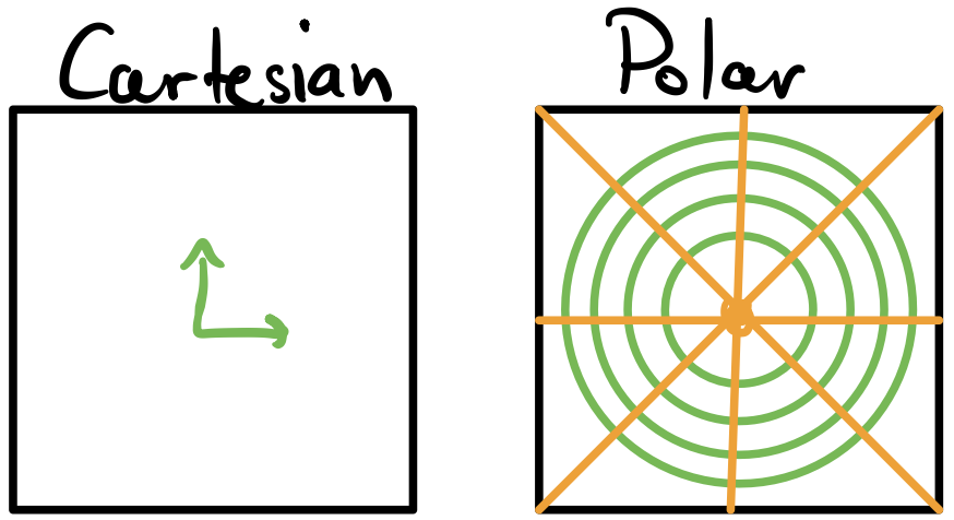
In Cartesian coordinates, it’s pretty clear to see that the components of the basis don’t change from point-to-point. However, in polar coordinates, this is not true. However, polar coordinates are just curved coordinates on a flat space! We need a way to differentiate an intrinsically curved space from just the choice of curved coordinates on that space.
Interestingly, the inverse can also be true: manifolds that appear to have curvature can actually be intrinsically flat! Consider a torus. At first glance, it appears to be a curved space, but that’s only extrinsically. As it turns out, we can show that the torus is actually intrinsically flat, specifically, it is the same as a square with the sides identified.
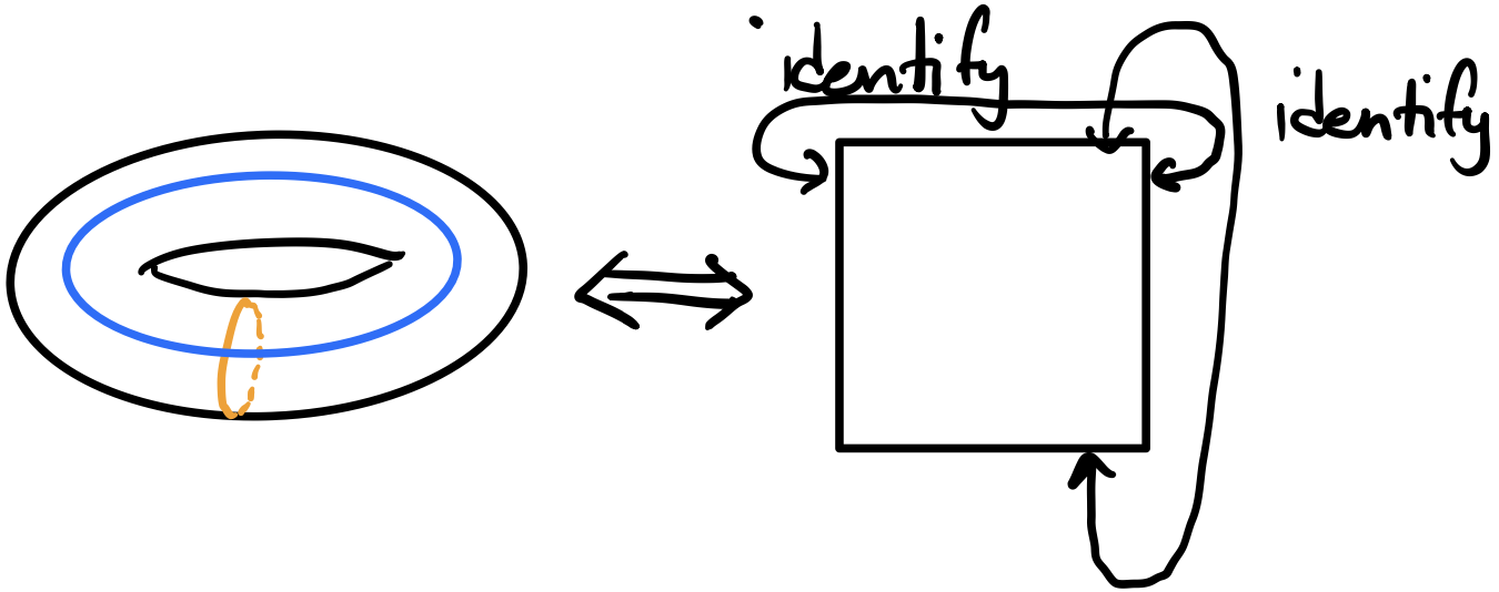
We can flatten a torus by cutting the torus into a cylinder and then cutting the cylinder in half and unrolling it. The sides are identified so the space “repeats”. On the other hand, there’s no way to cut a sphere into a flat space (in a way that preserves distances and angles).
So if we were a little bug on a torus, we would think our world was flat! We could construct a map of a torus on a piece of paper that perfectly preserves angles and distances. To complete the list of examples, a sphere, e.g., the surface of the Earth, is both extrinsically and intrinsically curved! We’ll see exactly how to prove this shortly.
So far, I’ve described curvature intuitively, but we need some equations to let us definitively differentiate a flat from a curved space. The key is to recall what we said about parallel transporting a vector from a start point to an end point: the final result depends on the path! Taking that same notion, what would happen if we parallel transported a vector in a little infinitesimal loop? In a flat space, either Cartesian or polar, the vector should be pointing in the same direction! But what if a space is not flat? Remember what happened for the sphere? When we parallel transported a vector in a loop, it wasn’t pointed in the same direction! Let’s take the same concept, but do it at a much smaller/infinitesimal scale so we can define a curvature at each point in space.
“Parallel transport around a little loop” is a bit too informal, so let’s use some equations to make this more concrete. Some texts take this too literally, but I think a better interpretation is to consider two vectors $A^\mu$ and $B^\nu$ and an arbitrary vector $V^\rho$ that we parallel transport along those two vectors. The mathematical way to represent this is with the commutator of the covariant derivative:
\[[\nabla_\mu, \nabla_\nu]V^\rho = \nabla_\mu \nabla_\nu V^\rho - \nabla_\nu \nabla_\mu V^\rho\]Intuitively, this is like transporting the vector to the far side of the loop and then back to the start again. The computation itself is fairly straightforward. Let’s first start by applying the outermost covariant derivative to the first term.
\[\nabla_\mu \nabla_\nu V^\rho - \nabla_\nu \nabla_\mu V^\rho = \p_\mu(\nabla_\nu V^\rho) - \Gamma_{\mu\nu}^\lambda\nabla_\lambda V^\rho + \Gamma_{\mu\sigma}^\rho\nabla_\nu V^\sigma - (\mu\leftrightarrow\nu)\\\]Recall that we’re applying $\nabla_\mu$ on the tensor $\nabla_\nu V^\rho$, which has one upper and one lower index so we need two connection coefficients. (You can think of this tensor as $(\nabla V)_\nu^\rho$ if that helps). As it turns out, the expansion of the second term is identical to the first except with the $\mu$s and $\nu$s swapped, which is denoted as $(\mu\leftrightarrow\nu)$. Don’t worry about those for now; we’ll expand them later. Now let’s expand the inner covariant derivative.
\[\p_\mu(\p_\nu V^\rho + \Gamma_{\mu\sigma}^\rho V^\sigma) - \Gamma_{\mu\nu}^\lambda(\p_\lambda V^\rho + \Gamma_{\lambda\sigma}^\rho V^\sigma) + \Gamma_{\mu\sigma}^\rho(\p_\nu V^\sigma + \Gamma_{\nu\lambda}^\sigma V^\lambda) - (\mu\leftrightarrow\nu)\\\]Now let’s multiple everything out, but be careful about the partial $\p_\mu$.
\[\p_\mu\p_\nu V^\rho + \p_\mu(\Gamma_{\mu\sigma}^\rho V^\sigma) - \Gamma_{\mu\nu}^\lambda\p_\lambda V^\rho - \Gamma_{\mu\nu}^\lambda\Gamma_{\lambda\sigma}^\rho V^\sigma + \Gamma_{\mu\sigma}^\rho\p_\nu V^\sigma + \Gamma_{\mu\sigma}^\rho\Gamma_{\nu\lambda}^\sigma V^\lambda - (\mu\leftrightarrow\nu)\\\]For the $\p_\mu(\Gamma_{\mu\sigma}^\rho V^\sigma)$ term, we have to expand it using the product rule!
\[\p_\mu\p_\nu V^\rho + \p_\mu\Gamma_{\mu\sigma}^\rho V^\sigma + \Gamma_{\mu\sigma}^\rho\p_\mu V^\sigma - \Gamma_{\mu\nu}^\lambda\p_\lambda V^\rho - \Gamma_{\mu\nu}^\lambda\Gamma_{\lambda\sigma}^\rho V^\sigma + \Gamma_{\mu\sigma}^\rho\p_\nu V^\sigma + \Gamma_{\mu\sigma}^\rho\Gamma_{\nu\lambda}^\sigma V^\lambda - (\mu\leftrightarrow\nu)\\\]Even though this equation already has a lot of terms, we’re ready to add in the other terms and see what cancels!
\[\begin{align*} \p_\mu\p_\nu V^\rho + \p_\mu\Gamma_{\mu\sigma}^\rho V^\sigma + \Gamma_{\mu\sigma}^\rho\p_\mu V^\sigma - \Gamma_{\mu\nu}^\lambda\p_\lambda V^\rho - \Gamma_{\mu\nu}^\lambda\Gamma_{\lambda\sigma}^\rho V^\sigma + \Gamma_{\mu\sigma}^\rho\p_\nu V^\sigma + \Gamma_{\mu\sigma}^\rho\Gamma_{\nu\lambda}^\sigma V^\lambda\\ -\p_\nu\p_\mu V^\rho - \p_\nu\Gamma_{\nu\sigma}^\rho V^\sigma - \Gamma_{\nu\sigma}^\rho\p_\nu V^\sigma + \Gamma_{\nu\mu}^\lambda\p_\lambda V^\rho + \Gamma_{\nu\mu}^\lambda\Gamma_{\lambda\sigma}^\rho V^\sigma - \Gamma_{\nu\sigma}^\rho\p_\mu V^\sigma - \Gamma_{\nu\sigma}^\rho\Gamma_{\mu\lambda}^\sigma V^\lambda\\ \end{align*}\]Remembering that partial derivatives commute, we can get rid of quite a few terms!
\[\require{cancel} \begin{align*} \cancel{\p_\mu\p_\nu V^\rho} + \p_\mu\Gamma_{\mu\sigma}^\rho V^\sigma + \bcancel{\Gamma_{\mu\sigma}^\rho\p_\mu V^\sigma} - \Gamma_{\mu\nu}^\lambda\p_\lambda V^\rho - \Gamma_{\mu\nu}^\lambda\Gamma_{\lambda\sigma}^\rho V^\sigma + \xcancel{\Gamma_{\mu\sigma}^\rho\p_\nu} V^\sigma + \Gamma_{\mu\sigma}^\rho\Gamma_{\nu\lambda}^\sigma V^\lambda\\ -\cancel{\p_\nu\p_\mu V^\rho} - \p_\nu\Gamma_{\nu\sigma}^\rho V^\sigma - \xcancel{\Gamma_{\nu\sigma}^\rho\p_\nu V^\sigma} + \Gamma_{\nu\mu}^\lambda\p_\lambda V^\rho + \Gamma_{\nu\mu}^\lambda\Gamma_{\lambda\sigma}^\rho V^\sigma - \bcancel{\Gamma_{\nu\sigma}^\rho\p_\mu V^\sigma} - \Gamma_{\nu\sigma}^\rho\Gamma_{\mu\lambda}^\sigma V^\lambda\\ \end{align*}\]Nearly half of our terms cancel! Let’s examine the surviving terms. I’ve swapped dummy indices $\lambda\leftrightarrow\sigma$ for the last terms of each line so that the notation is more consistent.
\[\begin{align*} \p_\mu\Gamma_{\mu\sigma}^\rho V^\sigma - \Gamma_{\mu\nu}^\lambda\p_\lambda V^\rho - \Gamma_{\mu\nu}^\lambda\Gamma_{\lambda\sigma}^\rho V^\sigma + \Gamma_{\mu\lambda}^\rho\Gamma_{\nu\sigma}^\lambda V^\sigma\\ - \p_\nu\Gamma_{\nu\sigma}^\rho V^\sigma + \Gamma_{\nu\mu}^\lambda\p_\lambda V^\rho + \Gamma_{\nu\mu}^\lambda\Gamma_{\lambda\sigma}^\rho V^\sigma - \Gamma_{\nu\lambda}^\rho\Gamma_{\mu\sigma}^\lambda V^\sigma\\ \end{align*}\]There are a few interesting things to notice, especially with the middle two terms of each line. They can each be condensed back into a covariant derivative, but with a connection coefficient as a coefficient on the front.
\[\begin{align*} \p_\mu\Gamma_{\mu\sigma}^\rho V^\sigma - \Gamma_{\mu\nu}^\lambda(\nabla_\lambda V^\rho) + \Gamma_{\mu\lambda}^\rho\Gamma_{\nu\sigma}^\lambda V^\sigma\\ - \p_\nu\Gamma_{\nu\sigma}^\rho V^\sigma + \Gamma_{\nu\mu}^\lambda(\nabla_\lambda V^\rho) - \Gamma_{\nu\lambda}^\rho\Gamma_{\mu\sigma}^\lambda V^\sigma\\ \end{align*}\]Yet another condensation we can do is to look at each term in the middle of each line. They’re almost identical except the $\mu$ and $\nu$ are swapped! This is exactly twice the commutator of the indices!
\[\p_\mu\Gamma_{\mu\sigma}^\rho V^\sigma + \Gamma_{\mu\lambda}^\rho\Gamma_{\nu\sigma}^\lambda V^\sigma - \p_\nu\Gamma_{\nu\sigma}^\rho V^\sigma - \Gamma_{\nu\lambda}^\rho\Gamma_{\mu\sigma}^\lambda V^\sigma - 2\Gamma_{[\mu\nu]}^\lambda\nabla_\lambda V^\rho \\\]But remember that for a torsion-free metric, this terms cancels so we’re left with only the first four terms, that we can factor out the $V^\sigma$ since it was arbitrary (and we do a bit of rearranging).
\[(\p_\mu\Gamma_{\mu\sigma}^\rho - \p_\nu\Gamma_{\nu\sigma}^\rho + \Gamma_{\mu\lambda}^\rho\Gamma_{\nu\sigma}^\lambda - \Gamma_{\nu\lambda}^\rho\Gamma_{\mu\sigma}^\lambda) V^\sigma\]With some inspection, the tensor in the parentheses seems to have one upper and three lower indices. We define this as the Riemann tensor, which tells us the curvature (at a point) of a space.
\[R_{\sigma\mu\nu}^\rho = \p_\mu\Gamma_{\mu\sigma}^\rho - \p_\nu\Gamma_{\nu\sigma}^\rho + \Gamma_{\mu\lambda}^\rho\Gamma_{\nu\sigma}^\lambda - \Gamma_{\nu\lambda}^\rho\Gamma_{\mu\sigma}^\lambda\]We went through several stages of equations to get here, but remember that we were trying to see what happens if we parallel transported a vector along a little infinitesimal loop. The final result is that the parallel transported vector is linearly transformed by the Riemann tensor! To see this more clearly, let me group the indices a bit differently: $(R_\sigma^\rho)_{\mu\nu}$. The first upper and lower indices together represent a linear transform, just like a matrix linearly transforms a vector. The last two lower indices tell us in which directions are we parallel transporting the vector along a little loop.
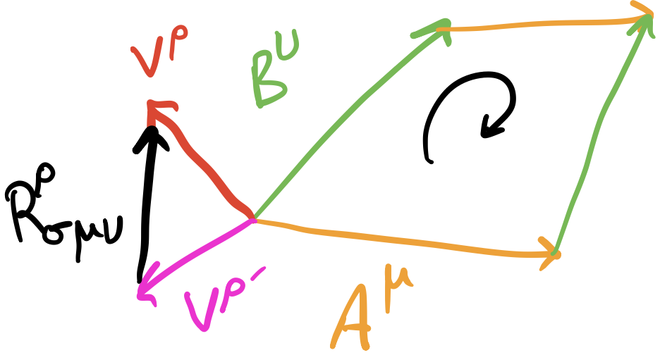
Similar to torsion, suppose we have two vectors $A^\mu$ and $B^\nu$ that we parallel transport into each other to make a closed loop (we’re assuming no torsion). Then if we have a vector $V^\rho$ that we move around in that little loop, we’ll end up with $V^{\rho’}$ that’s related to the original $V^\rho$ we started with by a linear transform. That linear transform that relates the two is what we call the Riemann tensor $R_{\sigma\mu\nu}^\rho$.
There are a few more things to note about this tensor. First of all, from the derivation, we can see that it’s antisymmetric in its last two lower indices. Imagine if we went around the loop in the other way and swapped $\mu$ and $\nu$ right from the beginning. Another important property is that it really does tell us if a space is flat or not because it’s written in terms of the derivatives of the connection, which, canonically, is written in terms of the metric. So this is effectively looking at second derivatives of the metric, similar to how curvature in a flat space looks at second derviatives. In Cartesian coordinates, we can immediately see that $R_{\sigma\mu\nu}^\rho=0$ everywhere.
As it turns out, there’s a theorem that says we can find a coordinate system in which the metric components are constant if and only if the Riemann tensor vanishes everywhere. From the above examples, it’s easy to show the forward implication of that theorem, but it’s a bit more work to show the backwards implication. I think the forward implication is more commonly used so I’ll skip the backwards implication and refer you to Sean Carroll’s book on general relativity.
In terms of components, navïely, we might think it has $n^4$ components since there are four indices, but, with the symmetries, we actually have much fewer components. The first symmetry we already saw: antisymmetric in the last two lower indices. There are more symmetries, but they are easier to discover if we lower the single upper index.
\[R_{\rho\sigma\mu\nu} = g_{\rho\lambda}R_{\sigma\mu\nu}^\lambda\]Let’s expand this out, but we’re going to use a special set of coordinates called Riemann normal coordinates. They’re a set of coordinates such that $\partial_{\sigma}g_{\mu\nu}=0$. A consequence of this (that you can verify yourself) is that all of the connection coefficients themselves are zero. However, this doesn’t mean the derivatives of the connection coefficients are zero so we still have to keep those.
\[\require{cancel} \begin{align*} R_{\rho\sigma\mu\nu} &= g_{\rho\lambda}R_{\sigma\mu\nu}^\lambda\\ &= g_{\rho\lambda}(\p_\mu\Gamma_{\mu\sigma}^\lambda- \p_\nu\Gamma_{\nu\sigma}^\lambda + \cancelto{0}{\Gamma_{\mu\lambda}^\lambda\Gamma_{\nu\sigma}^\lambda} - \cancelto{0}{\Gamma_{\nu\lambda}^\lambda\Gamma_{\mu\sigma}^\lambda)}\\ &= g_{\rho\lambda}(\p_\mu\Gamma_{\mu\sigma}^\lambda- \p_\nu\Gamma_{\nu\sigma}^\lambda)\\ \end{align*}\]Now we can expand the connection coefficients in terms of the metric (since we’re assuming a Levi-Civita connection):
\[\begin{align*} &= g_{\rho\lambda}(\p_\mu\Gamma_{\mu\sigma}^\lambda- \p_\nu\Gamma_{\nu\sigma}^\lambda)\\ &= g_{\rho\lambda}\Bigg(\p_\mu\Big[\frac{1}{2}g^{\lambda\tau}(\p_\nu g_{\sigma\tau} + \p_\sigma g_{\tau\nu} - \p_\tau g_{\nu\sigma})\Big] - \p_\nu\Big[\frac{1}{2}g^{\lambda\tau}(\p_\mu g_{\sigma\tau} + \p_\sigma g_{\tau\mu} - \p_\tau g_{\mu\sigma})\Big]\Bigg)\\ &= \frac{1}{2}g_{\rho\lambda}\Bigg(\p_\mu\Big[g^{\lambda\tau}(\p_\nu g_{\sigma\tau} + \p_\sigma g_{\tau\nu} - \p_\tau g_{\nu\sigma})\Big] - \p_\nu\Big[g^{\lambda\tau}(\p_\mu g_{\sigma\tau} + \p_\sigma g_{\tau\mu} - \p_\tau g_{\mu\sigma})\Big]\Bigg)\\ \end{align*}\]We have to expand out the inner partials $\p_\mu$ and $\p_\nu$ using the product rule, but remember that we’re in Riemann normal coordinates so the partials of the metric tensor and inverse metric tensor are zero $\p_\mu g^{\lambda\tau}=0$. So we can just apply the partial on the second term and factor out the $g^{\lambda\tau}$ to the front.
\[= \frac{1}{2}g_{\rho\lambda}g^{\lambda\tau}\Bigg(\p_\mu(\p_\nu g_{\sigma\tau} + \p_\sigma g_{\tau\nu} - \p_\tau g_{\nu\sigma}) - \p_\nu(\p_\mu g_{\sigma\tau} + \p_\sigma g_{\tau\mu} - \p_\tau g_{\mu\sigma})\Bigg)\]The partials can distribute through as well.
\[= \frac{1}{2}g_{\rho\lambda}g^{\lambda\tau}(\p_\mu\p_\nu g_{\sigma\tau} + \p_\mu\p_\sigma g_{\tau\nu} - \p_\mu\p_\tau g_{\nu\sigma} - \p_\nu\p_\mu g_{\sigma\tau} + \p_\nu\p_\sigma g_{\tau\mu} - \p_\nu\p_\tau g_{\mu\sigma})\]The partials commute so we can cancel out the first and fourth terms.
\[= \frac{1}{2}g_{\rho\lambda}g^{\lambda\tau}(\p_\mu\p_\sigma g_{\tau\nu} - \p_\mu\p_\tau g_{\nu\sigma} + \p_\nu\p_\sigma g_{\tau\mu} - \p_\nu\p_\tau g_{\mu\sigma})\]Finally, recall that $g_{\rho\lambda}g^{\lambda\tau}=\delta_\rho^\tau$ so we can substitute any lower $\tau$ with a $\rho$, and we’re left with the final result.
\[R_{\rho\sigma\mu\nu} = \frac{1}{2}(\p_\mu\p_\sigma g_{\rho\nu} - \p_\mu\p_\rho g_{\nu\sigma} + \p_\nu\p_\sigma g_{\rho\mu} - \p_\nu\p_\rho g_{\mu\sigma})\]From these terms, there are two symmetries we can see (by the fact the metric is symmetric and the partials commute). The first is that the tensor is antisymmetric in the first two indices.
\[R_{\rho\sigma\mu\nu} = -R_{\sigma\rho\mu\nu}\]Also, the tensor is invariant if we swap the first pair with the last pair of indices.
\[R_{\rho\sigma\mu\nu} = R_{\mu\nu\rho\sigma}\]You can convince yourself of these by substituting (and carefully changing indices around!) to find that things cancel or match up. There really isn’t much insight or practice gained from showing you that so I’ll just skip it. The last property is that if we cycle the last three indices completely and take the sum, everything cancels!
\[R_{\rho\sigma\mu\nu} + R_{\rho\mu\nu\sigma} + R_{\rho\nu\sigma\mu} = 0\]With some more index acrobatics, we can show that cyclical permutations are equivalent to taking a multi-index antisymmetry:
\[R_{\rho[\sigma\mu\nu]} = 0\](You can verify this yourself, but it’s not a very interesting calculation to do so I’ve also skipped this.) Note that we haven’t done anything non-tensorial here, even though we’ve used the connection coefficients.
Now we can use these symmetries to figure out the number of components. Using the first antisymmetry, the pairs of indices can only take the values $\binom{n}{2}$. To see this, consider $n=4$ (as commonly used in general relativity!). Because of the antisymmetry, the only unique values of the indices are $01$, $02$, $03$, $12$, $13$, $23$. The diagonal values vanish and the other side of the diagonal is repeated. Hence, we have $n$ choose $2$, in combinatorial syntax.
\[m = \binom{n}{2} = \frac{n(n-1)}{2}\]Now we can factor that into the second symmetry that says the first and second pair are swappable. For a symmetric matrix, we have $\frac{m(m+1)}{2}$ independent values, but that’s on top of the antisymmetry, which is why I used $m$ again. Substituting in terms of $n$, we can get the following (I’m skipping the algebra because it’s just algebra).
\[\frac{m(m+1)}{2} = \frac{n^4-2n^3+3n^2-2n}{8}\]Note that this is for the entire tensor so we need to subtract out additional constraints. Now to account for the cyclic permutation, using the same binomial syntax, we get $\binom{n}{4}$ because we’re fixing four indices. The permutation of the last three fixes the three, but the fourth one at the beginning also has to be subtracted else the relation devolves into the first and second symmetries.
\[\binom{n}{4} = \frac{n^4-6n^3+11n^2-6n}{24}\]This constrains the degrees of freedom from the general case of the first one so we subtract them to get the final result.
\[\frac{n^4-2n^3+3n^2-2n}{8} - \frac{n^4-6n^3+11n^2-6n}{24} = \frac{n^2(n^2 - 1)}{12}\](Yet again, I’ve skipped over the algebra because it’s not very interesting.) Finally we’re left with the number of independent components of the Riemann tensor with all of the symmetries accounted for! It’s certainly smaller than $n^4$, but it’s also not that small. For $n=4$, we have 20 independent components.
There’s just one last property regarding the Riemann tensor we need to discuss before we can simplify it into something easier to use. We can consider the derivative of the lowered Riemann (also in Riemann normal coordinates so there’s no connection coefficient term).
\[\begin{align*} \nabla_\lambda R_{\rho\sigma\mu\nu} &= \p_\lambda R_{\rho\sigma\mu\nu}\\ &= \frac{1}{2}\p_\lambda (\p_\mu\p_\sigma g_{\rho\nu} - \p_\mu\p_\rho g_{\nu\sigma} + \p_\nu\p_\sigma g_{\rho\mu} - \p_\nu\p_\rho g_{\mu\sigma})\\ &= \frac{1}{2}(\p_\lambda \p_\mu\p_\sigma g_{\rho\nu} - \p_\lambda \p_\mu\p_\rho g_{\nu\sigma} + \p_\lambda \p_\nu\p_\sigma g_{\rho\mu} - \p_\lambda \p_\nu\p_\rho g_{\mu\sigma})\\ \end{align*}\]If we consider cyclical permutations of the first three indices, everything cancels!
\[\nabla_\lambda R_{\rho\sigma\mu\nu} + \nabla_\rho R_{\sigma\lambda\mu\nu} + \nabla_\sigma R_{\lambda\rho\mu\nu} = 0\]Like with the symmetry with cyclical permutations of the last three indices, we can use an equivalent antisymmetry.
\[\nabla_{[\lambda} R_{\rho\sigma]\mu\nu} = 0\]The above property is called the Bianchi identity and it’s actually used to prove an important property of the Einstein Field Equations used in general relativity.
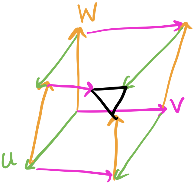
One geometric interpretation of the Bianchi Identity that I really like is the ability/inability to close a parallelepiped. Suppose we have three vectors $U$, $V$, and $W$. If we parallel transport each in the direction of each other, we’ll get a parallelepiped. The Bianchi Identity measures the ability of the ends of the vectors to close into a closed parallelepiped.
Even for small dimensionalities, the Riemann tensor has a lot of components! Practically speaking, we don’t often have to deal with this tensor directly. Instead, we can deal with a smaller tensor formed from a contraction of the Riemann tensor called the Ricci tensor.
\[R_{\mu\nu} = R_{\mu\lambda\nu}^\lambda\]In fact, we can contract it even further to get a scalar called the Ricci scalar.
\[R = R_\mu^\mu= g^{\mu\nu}R_{\mu\nu}\]As with the Riemann tensor, I also want to provide some illustrative intuition behind both of these quantities. (I won’t go through the exact proofs since that requires setting up some more machinery.) One interpretation I really like is John Baez’s coffee grounds. Imagine a ball of comoving coffee grounds on the manifold; “comoving” just means each individual coffee particle is at rest relative to all of the others so the whole group moves as a single coffee ground blob. In a flat space, the shape and size remain the same no matter how we move around the manifold. But, on a curved manifold, the ball might expand, collapse, rotate, or deform in all kinds of different ways. This is because each individual coffee ground doesn’t follow the same geodesic. The Ricci tensor measures only the change in volume of our coffee grounds. There is an other tensor called the Weyl tensor that measures the deformation.
The Ricci scalar, sometimes called scalar curvature, measures how the volume of the coffee ground blob differs from flat space. A positive scalar curvature is like a sphere. As we’ll see, a sphere has positive curvature everywhere, and geodesics tend to “bend apart” on a sphere. On the other hand, a negative curvature is like a saddle.
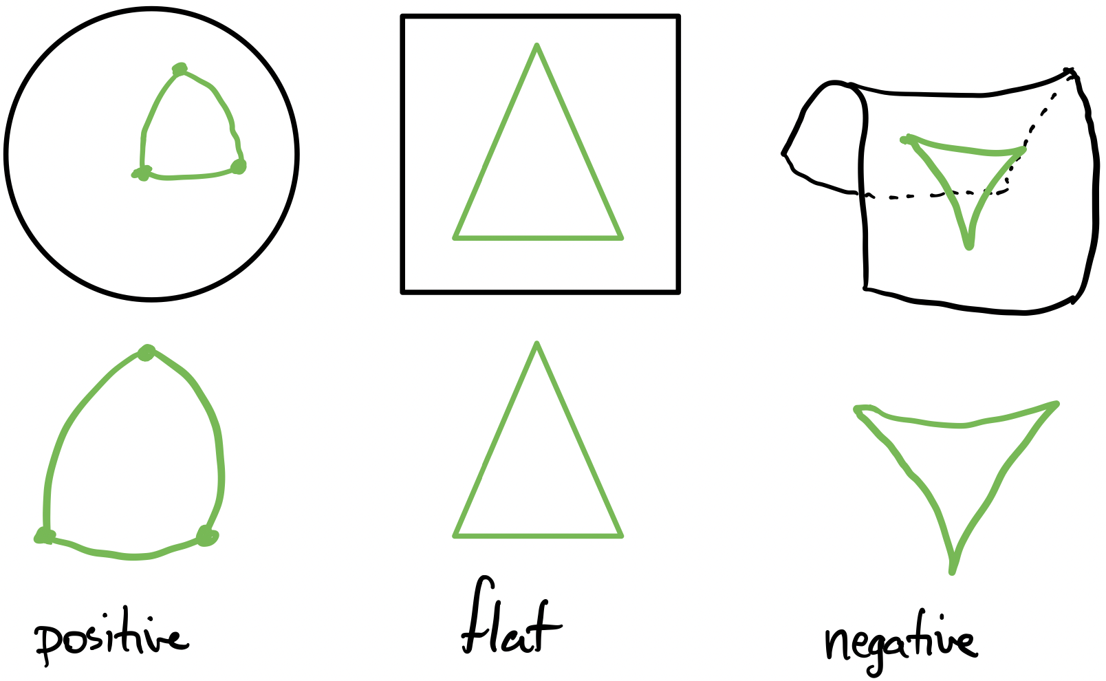
With a positive scalar curvature, like a sphere, the edges of a triangle will “bow outward”. This is the reason we need to use the Haversine Formula when we look at angles and distance on the surface of the Earth. In a flat space, a triangle is simply a triangle. With a negative scalar curvature, like with a saddle, the edges of a triangle will “bow inward”.
To see a practical application of the Ricci tensor and scalar to general realtivity, there’s a little computation we have to do first. Taking the Bianchi identity a step further, we can contract it twice on the Bianchi identity to write it in terms of the Ricci tensor and Ricci scalar.
\[\begin{align*} g^{\nu\sigma}g^{\mu\lambda}(\nabla_\lambda R_{\rho\sigma\mu\nu} + \nabla_\rho R_{\sigma\lambda\mu\nu} + \nabla_\sigma R_{\lambda\rho\mu\nu}) &= 0\\ g^{\nu\sigma}g^{\mu\lambda}(\nabla_\lambda R_{\mu\nu\rho\sigma} + \nabla_\rho R_{\mu\nu\sigma\lambda} + \nabla_\sigma R_{\lambda\rho\mu\nu}) &= 0\\ g^{\nu\sigma}g^{\mu\lambda}(\nabla_\lambda R_{\mu\nu\rho\sigma} - \nabla_\rho R_{\nu\mu\sigma\lambda} + \nabla_\sigma R_{\lambda\rho\mu\nu}) &= 0\\ g^{\nu\sigma}(\nabla^\mu R_{\mu\nu\rho\sigma} - \nabla_\rho R_{\nu\mu\sigma}^\mu + \nabla_\sigma R_{\rho\mu\nu}^\mu) &= 0\\ g^{\nu\sigma}(\nabla^\mu R_{\mu\nu\rho\sigma} - \nabla_\rho R_{\nu\sigma} + \nabla_\sigma R_{\rho\nu}) &= 0\\ \nabla^\mu R_{\mu\nu\rho}^\nu - \nabla_\rho R_{\nu}^\nu + \nabla^\nu R_{\rho\nu} &= 0\\ \nabla^\mu R_{\mu\rho} - \nabla_\rho R + \nabla^\nu R_{\rho\nu} &= 0\\ \nabla^\mu R_{\mu\rho} - \nabla_\rho R + \nabla^\mu R_{\mu\rho} &= 0\\ 2\nabla^\mu R_{\mu\rho} - \nabla_\rho R &= 0\\ \nabla^\mu R_{\mu\rho} - \frac{1}{2}\nabla_\rho R &= 0\\ \nabla^\mu R_{\mu\rho} &= \frac{1}{2}\nabla_\rho R\\ \end{align*}\]Between the first two equations, I used the second symmetry on the first and second terms. From the second and third equations, I used the first antisymmetry on the second term. The rest follow from raising the tensors and forming the Ricci tensor and Ricci scalar. Note that we can raise the index on a covariant derivative (rather than a partial) because of metric compatibility.
Now suppose we define the Einstein tensor in terms of the Ricci tensor and scalar as the following.
\[G_{\mu\nu} \equiv R_{\mu\nu} - \frac{1}{2}R g_{\mu\nu}\](Note that this tensor is also symmetric because the Ricci tensor and the metric are also symmetric!) Applying to the above Bianchi identity, we can see the following property is true.
\[\begin{align*} \nabla^\mu G_{\mu\nu} &= 0\\ \nabla^\mu (R_{\mu\nu} - \frac{1}{2}R g_{\mu\nu}) &= 0\\ \nabla^\mu R_{\mu\nu} - \frac{1}{2}\nabla^\mu g_{\mu\nu} R &= 0\\ \nabla^\mu R_{\mu\nu} - \frac{1}{2}\nabla_\nu R &= 0\\ \end{align*}\]Note that the final line corresponds to the second-to-last line of the Bianchi identity above. As it turns out, this property corresponds to the conservation of energy and momentum in general relativity! In fact, the Einstein tensor is actually the left half of the Einstein Field Equations (EFE) that tell us how the geometry of a space is affected by the energy-momentum of that space.
Example: The 2-Sphere
So far, we’ve set up a ton of machinery, so let’s put it into practice on a canonical example: the two-sphere $S^2$!
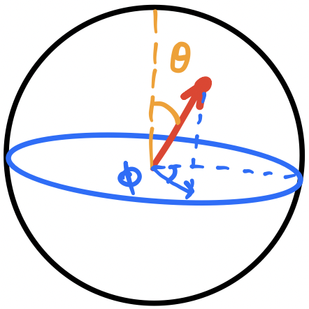
We’ll define intrinsic spherical coordinates like a physicist such that the polar angle, i.e., the angle with respect to the $z$-axis is $\theta$ and the azimuthal angle, i.e., the angle in the $xy$-plane from the $x$-axis, is $\phi$.
The metric for a two-sphere requires only two intrinsic coordinates. Think about the Earth: we only need a latitude and longitude to specify a coordinate on the surface. To see this, let’s start with the spherical coordinate metric in a flat space.
\[\d s^2 = \d r^2 + r^2 \d\theta^2 + r^2\sin^2\theta\d\phi^2\]However, if we’re on a sphere of a constant radius, note that $\d r^2$ vanishes and we’re left with an intrinsic metric on a sphere.
\[\d s^2 = r^2(\d\theta^2 + \sin^2\theta\d\phi^2)\]Visually, treat $\d s^2$ as a little slice along the sphere, in terms of a $\theta$ and $\phi$. We can write the components of the metric and inverse metric tensor in matrix form.
\[\begin{align*} g_{ij} &= \begin{bmatrix}1 & 0\\ 0 & \sin^2\theta \end{bmatrix}\\ g^{ij} &= \begin{bmatrix}1 & 0\\ 0 & \frac{1}{\sin^2\theta} \end{bmatrix}\\ \end{align*}\](Recall that the inverse of a diagonal metric is just the inverse of the components.) From these, we can compute the connection coefficients. It’s just the algebra of plugging the connection coefficients into the equation and churning them out. Remember that the bottom two indices are symmetric so we don’t have to compute them twice. Also, the off-diagonals of the metric and its inverse are zero so this should make it a bit easier. The only non-zero connection coefficients are the following.
\[\begin{align*} \Gamma^\theta_{\phi\phi} &= -\cos\theta\sin\theta\\ \Gamma^\phi_{\theta\phi} = \Gamma^\phi_{\phi\theta} &= \cot\theta\\ \end{align*}\]While we’re at it, we can compute the Ricci tensor. (This is also just algebra.)
\[\begin{align*} R_{\theta\theta} &= 1\\ R_{\theta\phi} = R_{\phi\theta} &= 0\\ R_{\phi\phi} &= r^2\sin^2\theta\\ \end{align*}\]And finally we can compute the Ricci scalar.
\[R = \frac{2}{r^2}\]From this, we see that the Ricci scalar is constant across the sphere and positive. This makes sense since neighboring geodesics tend to “bow” outwards and “inflate”. On the other hand, if we had added some “noise” to the metric, then this wouldn’t be the case. One interesting thing to note is that the scalar curvature increases as the radius decreases. One interesting application is that we can model some kinds of black hole’s event horizons as sphere. And, as it turns out, the strength of tidal forces is inversely proportional to the scalar curvature. In other words, a black hole with a very large event horizon doesn’t have as strong tidal forces. For the supermassive black hole at the center of our Milky Way galaxy, we could toss anything in without it being ripped apart by tidal forces.
Another, more interesting, thing to consider is geodesics on the sphere. This is particular interesting because, if we wanted to find the shortest path between two points on the Earth, the geodesic tell us exactly that! Let’s start by rewriting the geodesic equation.
\[\frac{\d^2 x^\mu}{\d\lambda^2} + \Gamma_{\sigma\rho}^\mu\frac{\d x^\sigma}{\d\lambda}\frac{\d x^\rho}{\d\lambda} = 0\]Recall that these are actually a set of 2nd order differential equations in $\mu$. Since we have two coordinates $\theta$ and $\phi$, we’ll have two equations. We can also simplify the equations since there are only two unique, non-zero connection coefficients.
\[\begin{align*} \frac{\d^2 x^\theta}{\d\lambda^2} + \Gamma_{\phi\phi}^\theta\frac{\d x^\phi}{\d\lambda}\frac{\d x^\phi}{\d\lambda} &= 0\\ \frac{\d^2 x^\phi}{\d\lambda^2} + \Gamma_{\theta\phi}^\phi\frac{\d x^\theta}{\d\lambda}\frac{\d x^\phi}{\d\lambda} +\Gamma_{\phi\theta}^\phi\frac{\d x^\phi}{\d\lambda}\frac{\d x^\theta}{\d\lambda}&= 0\\ \end{align*}\]But remember that the connection coefficients are symmetric so the last two terms in the second equation are the same.
\[\begin{align*} \frac{\d^2 x^\theta}{\d\lambda^2} + \Gamma_{\phi\phi}^\theta\frac{\d x^\phi}{\d\lambda}\frac{\d x^\phi}{\d\lambda} &= 0\\ \frac{\d^2 x^\phi}{\d\lambda^2} + 2\Gamma_{\theta\phi}^\phi\frac{\d x^\theta}{\d\lambda}\frac{\d x^\phi}{\d\lambda} &= 0\\ \end{align*}\]Now let’s plug in the values for the connection coefficients.
\[\begin{align*} \frac{\d^2 x^\theta}{\d\lambda^2} -\cos\theta\sin\theta\frac{\d x^\phi}{\d\lambda}\frac{\d x^\phi}{\d\lambda} &= 0\\ \frac{\d^2 x^\phi}{\d\lambda^2} + 2\cot\theta\frac{\d x^\theta}{\d\lambda}\frac{\d x^\phi}{\d\lambda} &= 0\\ \end{align*}\]These are a set of paired 2nd order differential equations that are too difficult to solve in general. Fortunately, the sphere has a lot of symmetries so, even if we restrict the solution, we can use those symmetries to produce general solutions. For now, let’s fix a lattitude $\theta=\tilde{\theta}$ so we have the equations $x^\theta(\lambda)=\tilde{\theta}, x^\phi(\lambda)=\alpha\lambda + \beta$ where $\alpha$ and $\beta$ are just constants that represent path around the lattitude. (We could ignore $\beta$, but I left it in for completeness.) Now let’s compute the first and second order derivatives needed for the geodesic equation.
\[\begin{align*} \frac{\d x^\theta}{\d\lambda} = 0 &, \frac{\d x^\phi}{\d\lambda} = \alpha\\ \frac{\d^2 x^\theta}{\d\lambda^2} = 0 &, \frac{\d^2 x^\phi}{\d\lambda^2} = 0\\ \end{align*}\]Now we can plug these into the geodesic equation and substitute $\theta=\tilde{\theta}$.
\[\begin{align*} 0 - \cos\tilde{\theta}\sin\tilde{\theta}\cdot\alpha^2 &= 0\\ 0 + 2\cot\tilde{\theta}\cdot 0\cdot\alpha &= 0\\ \end{align*}\]The second equation is just $0=0$ so we can ignore that so we can just focus on the first one.
\[- \cos\tilde{\theta}\sin\tilde{\theta}\cdot\alpha^2 = 0\]The goal is to set $\tilde{\theta}$ and $\alpha$ such that the equation is also $0=0$. The easiest thing to do seems to be to set $\alpha=0$. But if we do that, the resulting equations become $x^\theta(\lambda)=\tilde{\theta}, x^\phi(\lambda)=\beta$, which is just a fixed point on the sphere. Let’s try to set $\sin\tilde{\theta}=0$. In this case, $\tilde{\theta}=0$ or $\tilde{\theta}=\pi$. The resulting equations become $x^\theta(\lambda)=0, x^\phi(\lambda)=\alpha\lambda+\beta$, but this is also just a point because $x^\theta(\lambda)=0$ and $x^\theta(\lambda)=\pi$ are the North and South Poles.
Instead, let’s try to set $\cos\tilde{\theta}=0$, which means $\tilde{\theta}=\frac{\pi}{2}$. The equations become $x^\theta(\lambda)=\frac{\pi}{2}, x^\phi(\lambda)=\alpha\lambda+\beta$. This represents a path along the equator! This kind of circle is called a great circle: a circle on a sphere where the center of the circle is the center of the sphere. Using the rotational symmetry of the sphere, all geodesics on a sphere are great circles. In other words, the shortest distance between any two points on a sphere is the great circle that contains those two points. (There are actually two directions, but we can simply pick the shortest one.) With this, we have shown that geodesics on spheres are all great circles using the geodesic equation. An alternative to finding geodesics with the geodesic equation is to use calculus of variations and the Euler-Lagrange equations, and that’s sometimes easier (maybe I’ll explain that in another post!), but this is also a valid way of finding geodesics.
Conclusion
We’ve covered a lot of topics in this post, eventually culminating in answering a deceptively simple question: “how do we know if a space is flat?”. We saw that this was not an easy question when manifolds and intrinsic geometry was involved! To answer that question, we had to build up to it piece-by-piece, starting with a good intrinsic derivative operator, then discussing how to compare vectors on a manifold, and ending on curvature with a peek into general relativity. Here are some of the core concepts we learned:
- The covariant derivative is a way to compute derivatives on a manifold that accounts for the changing basis using the connection coefficients. The connection coefficients do not transform like tensors intentionally, to cancel out the non-tensorial part of the partial derivative.
- Parallel transport is a way to move a vector along a curve so that it stays “as straight as possible.” On a manifold, there is no way to compare vectors at different points and how the vector changes depends on the path.
- A geodesic is the generalization of straight lines in on a manifold. It is the curve that parallel transports its own tangent vector. We can construct geodesics at a point by using the exponential map to project a tangent vector into a curve on the manifold.
- The Riemann tensor characterizes the intrinsic curvative of a manifold by parallel transporting a vector along a little loop and measure how much it changes. If the Riemann tensor is zero everywhere, then there exists a coordinate system where the metric is flat.
- The Ricci tensor is a useful contraction of the Riemann tensor that shows how a small group of neighboring geodesics change in volume as they move about the manifold. The Ricci scalar is a scalar way to measure that change.
That’s all! In this set of posts, we’ve learned all about manifolds and how to do calculus on them 😀