Neural Nets - Part 2: From Perceptrons to Modern Artificial Neurons
In the previous post, we motivated perceptrons as the smallest and simplest form of artificial neuron inspired by biological neurons. It consumed some inputs, applied a threshold function, and produced a binary output. While it did seem to model biology, it wasn’t quite as useful for machines. We applied some changes to make it more machine-friendly and applied it to learning logic gates. We even stacked them to form a 2-layer deep perceptron to solve the XOR gate problem! However, the weights and biases we “solved” for were just by inspection and logical reasoning. In practice, neural networks can have millions of parameters so this strategy is not really feasible.
In this post, we’ll learn how to automatically solve for the parameters of a simple neural model. In doing so, we’ll make a number of modifications that will evolve the perceptron into a more modern artificial neuron that we can use as a building block for wider and deeper neural networks. Similar to last time, we’ll implement this new artificial neuron using Python and numpy.
Gradient Descent
In the past, we solved for the weights and biases by inspection. This was feasible since logic gates are human-interpretable and the number of parameters was small. Now consider trying to come up with a network for trying to detect a mug in an image. This is a much more complicated task that required understand what a “mug” even is. What do the weights correspond to, and how would we set them manually? In practice, we have very wide and large networks with hundreds of thousands or even millions and billions of parameters, and we need a way to find appropriate values for these to solve our objective, e.g., emulating logic gates or detecting mugs in images.
Fortunately for us, there already exists a field of mathematics that’s been around for a long time that specializes in solving for these parameters: numerical optimization (or just optimization for short). In an optimization problem, we have a mathematical model, often represented as a function like $f(x; \theta)$ with some inputs $x$ and parameters $\theta$, and the goal is to find the values of the parameters such that some objective function $C$ satisfies some criteria. In most cases, we’re minimizing or maximizing it; in the former case, this objective function is sometimes called a cost/loss/error function (all are interchangeable), and in the latter case it is sometimes called a utility/reward function (all are interchangeable). There’s already a vast literature of numerical optimization techniques to draw from so we should try to leverage these rather than building something from scratch.
More specifically, in the case of our problem, we have a neural network represented by a function $f(x;W,b)$ that accepts input $x$ and is parameterized by its weights $W$ and biases $b$. But to use the framework of numerical optimization and its techniques, we need an objective function. In other words, how do we quantify what a “good” model is? In our classification task, we want to ensure that the output of the model is the same as the desired training label for all training examples so we can intuitively think of this as trying to minimize the mistakes of our model output from the true training label.
\[C = \displaystyle\sum_i \vert f(x_i;W,b) - y_i\vert\]Notice we used the absolute value since any difference will increase our cost; verify this for yourself (for a single training example) that when the output of the model is different from $y_i$, $C > 0$ and when and output is the same as $y_i$, $C = 0$. This cost function is also sometimes called mean absolute error (MAE). (Sometimes we’ll see a $\frac{1}{N}$, where $N$ is the number of training examples, in front of the sum but this is just a constant factor that makes the maths easier so we can omit it without any issue.) We only get $C=0$ if, for every training example, $f(x_i;W,b) = y_i$, i.e., our model always classifies correctly. Now we have our model and our cost function so we can try to figure out which optimization approach is well-suited for our problem.
One bifurcation of the numerical optimization field is gradient-free and gradient-based methods. Recall from calculus that a gradient measures the rate-of-change of a function with respect to all of its inputs. This extra information in addition to the objective function itself that, if we choose to use it, will have to be computed and maintained. So the former set of methods describes approaches where we don’t need this extra information and rely on just the values of the objective function itself. The latter describes a set of methods where we do use this extra information. In practice, gradient-based methods tend to work better for neural networks since they tend to converge to a better solution, i.e., they more quickly find the set of parameters with lower cost, but it should be noted there are techniques that optimize neural networks using gradient-free approaches as well.
The idea behind gradient-based methods is to compute a partial derivative of the cost function with respect to each parameter $\frac{\p C}{\p \theta_i}$ of the model. From calculus, we can arrange these partial derivatives in a vector called the gradient $\nabla_\theta C$. This quantity tells us how changes in a parameter $\theta_i$ correspond to changes in the cost function $C$; specifically, it tells us how to change $\theta_i$ to increase the value of $C$. Mathematically speaking, if we have a function of a single variable $C(\theta)$ and a little change in its inputs $\Delta\theta$, then $C(\theta + \Delta\theta)\approx C(\theta)+\frac{\p C}{\p\theta}\Delta\theta$; in other words, a little change in the input is mapped to a little change in the output, but proportional to how the cost function changes with respect to that little input: $\frac{\p C}{\p \theta}$. This is very useful because it can tell us in which direction to move $\theta_i$ such that the value of $C$ decreases, i.e., $-\frac{\p C}{\p \theta_i}$. Remember that in our ideal case, we want $C=0$ (we minimize cost functions and maximize reward functions), and the negative of the partial derivatives tell us exactly how to accomplish this. With this information, we can nudge the parameters $\theta$ using the gradient of the cost function.
\[\theta_i\gets\theta_i - \eta\displaystyle\frac{\p C}{\p \theta_i}\]or in vectorized form
\[\theta\gets\theta - \eta\nabla_\theta C\]Just like with perceptrons, we’ll have a learning rate $\eta$ that is a tuning parameter that tells us how much to adjust the current $\theta$ by. If we do this, we can find the values of the parameters such that the cost function is minimized! This optimization technique is called gradient descent.
(Note that I’ll be using a bit sloppy with my nomenclature and interchangeably say “partial derivative” and “gradient” but just remember the definition of the gradient of a function: the vector of all partial derivatives of the function with respect to each parameter.)
One intuitive way to visualize gradient descent is to think about $C$ is as an “elevation”, like on a topographic map and and the objective is to find the single lowest valley. Mathematically, we’re trying to find the global minima of the cost function. If we could analytically and tractably compute $C$ exactly with respect to all parameters and the entire dataset, then we could just use calculus to solve for the global minima and be finished perfectly! However, the complexity of neural networks along with the size of the datasets they’re often trained on makes this approach infeasible.
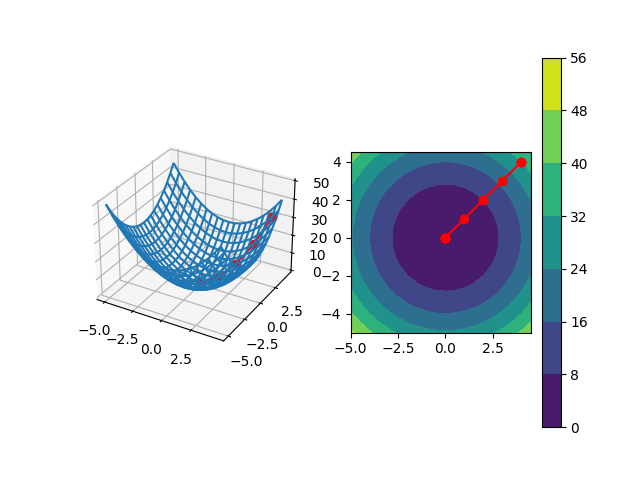
Suppose we have a very well-behaved cost function $C(x, y) = x^2+y^2$ with a single global minima. The idea behind gradient descent is to start at some random point $(x, y)$, e.g., $(5, 5)$ in this example, on this cost surface and incrementally move in a way such that we ultimately arrive at the lowest-possible point. The left figure shows the 3D mesh of the cost function (z axis is the value of the cost function for its x and y axis inputs) as well as the path that gradient descent will take us from the starting point $(5, 5)$ to the global minima at the origin. The right figure shows the same, but a top-down view where the colors represent the value of the cost function.
Instead, imagine we’re at some starting point on the cost surface. Using the negative of the gradient tells us how to move parameters from where we currently are to get to a slightly lower point on the cost surface from where we were. If the cost function is well-behaved, this should decrease our overall cost. We repeatedly do this until we’re at a point on the cost surface where, no matter which direction we nudge our parameters, the cost always increases. This is a minima! Depending on the cost function, we might have multiple local minima which are locally optimal within some bounds of the cost function, but they’re not optimal across the entire cost function; that would be the global minima, which is the best solution.
Another intuitive way to think about this is suppose someone took us hiking and we got lost. All we know is that there is a town in the valley of the mountain but there’s a thick fog so we’re unable to see far out. Rather than picking a random direction to walk in, we can look around (within the visibility of the fog) to see if the elevation goes downhill from where we currently are, and then move in that direction. While we’re moving, we’re constantly evaluating which direction would bring us downhill. We repeat until, no matter which direction we look, we’re always going uphill.
Let’s apply what we’ve learned so far to the same Iris dataset example we did last time! Let’s try to train our perceptron using gradient descent. We’ll use the cost function above and analytically compute the gradients to update the weights. However, we’ll run into an immediate problem: the Heaviside step function we’re using as an activation function. Recall its definition:
\[f(\theta)=\begin{cases} 1 & \theta \geq 0 \\ 0 & \theta < 0 \\ \end{cases}\]We’ll be computing a gradient, and this step function has a nonlinearity at 0. That alone isn’t a huge issue; the larger issue is that the gradient will be 0 since the output of the step function is constant and the derivative of a constant is always 0. We’ll get no parameter update from gradient descent, and our model won’t learn a thing! So this choice of activation function isn’t going to work; we need an activation function that actually has a gradient.
Rather than picking the step function, we can try to pick a differentiable function that looks just like a step function. Fortunately for us, there exists a whole class of functions call logistic functions that closely resemble this step function. One specific logistic curve is called the sigmoid.
\[\sigma(z) \equiv \frac{1}{1+e^{-z}}\]The function itself actually even looks like a smooth version of the step function!
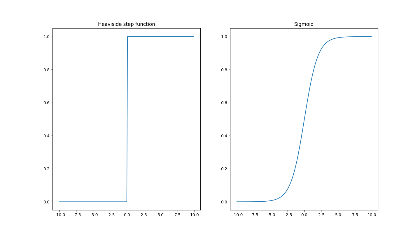
The sigmoid (right) can be considered a smooth version of the Heaviside step function (left) so it can be differentiated an infinite amount of times. Both map their unbounded input to a bounded output, but the nuance is that the step function bound is inclusive $[0, 1]$ while the sigmoid bound is exclusive $(0, 1)$ because of the asymptotes.
Note that if the input $z$ is very large and positive, then the sigmoid function asymptotes/saturates to $1$ and if the input is very large and negative, the sigmoid function asymptotes to $0$. In other words, it maps the unbounded real number line $(-\infty, \infty)$ to the bounded interval $(0, 1)$. The sigmoid is smooth in that we can take a derivative, and that little changes in the input will map to little changes in the output. In fact, the derivative of the sigmoid can be expressed in terms of the sigmoid itself (thanks to the properties of the $e$ in its definition!)
\[\sigma'(z) = \sigma(z)(1 - \sigma(z))\]It’s a good exercise to verify this for yourself! (Hint: rewrite $\sigma(z) = (1+e^{-z})^{-1}$ and use the power rule.)
Now let’s replace our step function with the sigmoid so we do end up with nonzero derivatives. Remember we’re trying to compute the gradient of the cost function with respect to the two weights $w_1$ and $w_2$ and the bias $b$. Substituting and expanding the cost function for a single training example, we get the following.
\[C = \vert \sigma(w_1 x_1 + w_2 x_2 + b) - y\vert\]Let’s start with computing $\frac{\p C}{\p w_1}$ and the other derivatives will follow. We’ll need to make liberal use of the chain rule; the way I remember it is “derivative of the outside with respect to the inside times the derivative of the inside $\frac{\d}{\d x}f(g(x)) = f’(g(x))g’(x)$. We’ll also need to know that the derivative of the absolute value function $f(x)=\vert x\vert$ is the sign function $\sgn(x)$ that returns 1 if the input is positive and -1 if the input is negative and is mathematically undefined if the input is 0, but practically, in this specific example, we can let $\sgn(0) = 0$. (Similar to the Heaviside step function, we can see this from plotting the absolute value function, looks like a ‘V’, and noting that both sides of the ‘V’ have a constant slope of $\pm 1$ depending on the side of the ‘V’.)
\[\begin{align*} \displaystyle\frac{\p C}{\p w_1} &= \frac{\p}{\p w_1} \vert \sigma(w_1 x_1 + w_2 x_2 + b) - y\vert \\ &= \sgn\big[\sigma(w_1 x_1 + w_2 x_2 + b) - y\big] \frac{\p}{\p w_1}\big[\sigma(w_1 x_1 + w_2 x_2 + b) - y\big]\\ &= \sgn\big[\sigma(w_1 x_1 + w_2 x_2 + b) - y\big] \frac{\p}{\p w_1}\sigma(w_1 x_1 + w_2 x_2 + b)\\ &= \sgn\big[\sigma(w_1 x_1 + w_2 x_2 + b) - y\big] \sigma'(w_1 x_1 + w_2 x_2 + b)\frac{\p}{\p w_1}\big[w_1 x_1 + w_2 x_2 + b\big]\\ &= \sgn\big[\sigma(w_1 x_1 + w_2 x_2 + b) - y\big] \sigma'(w_1 x_1 + w_2 x_2 + b)\frac{\p}{\p w_1}\big[w_1 x_1\big]\\ &= \sgn\big[\sigma(w_1 x_1 + w_2 x_2 + b) - y\big] \sigma'(w_1 x_1 + w_2 x_2 + b)x_1\\ &= \sgn(a - y) \sigma'(z)x_1\\ \end{align*}\]In the last step, we simplified by substituting back $z=w_1 x_1 + w_2 x_2 + b$ and $a=\sigma(z)$. Similarly, the other derivatives follow from this one with only minor changes in the last few steps so we can compute them all.
\[\begin{align*} \displaystyle\frac{\p C}{\p w_1} &= \sgn(a - y) \sigma'(z)x_1 \\ \displaystyle\frac{\p C}{\p w_2} &= \sgn(a - y) \sigma'(z)x_2 \\ \displaystyle\frac{\p C}{\p b} &= \sgn(a - y) \sigma'(z) \\ \end{align*}\]Another way to think about these derivatives that will be useful for implementation in code is expanding out the partials in accordance with the chain rule.
\[\begin{align*} \displaystyle\frac{\p C}{\p w_1} &= \displaystyle\frac{\p C}{\p a} \displaystyle\frac{\p a}{\p z}\displaystyle\frac{\p z}{\p w_1} \\ \displaystyle\frac{\p C}{\p w_2} &= \displaystyle\frac{\p C}{\p a} \displaystyle\frac{\p a}{\p z}\displaystyle\frac{\p z}{\p w_2} \\ \displaystyle\frac{\p C}{\p b} &= \displaystyle\frac{\p C}{\p a} \displaystyle\frac{\p a}{\p z}\displaystyle\frac{\p z}{\p b} \\ \end{align*}\]So the first two terms in each of these are the same, and it’s only the last term that we have to actually change. Now that we have these gradients computed analytically, we can get around to writing code!
A sketch of the general training algorithm is going to look like this.
- For each epoch
- For each training example $(x, y)$
- Perform a forward pass through the model $y = f(x)$
- Perform a backward pass to compute weight $\frac{\p C}{\p W_i}$ and bias $\frac{\p C}{\p b}$ gradients
- Update the weights and biases
- For each training example $(x, y)$
We refer to passing an input through the network to get an output as a forward pass and computing gradients as a backward pass because of the nature of how we perform both computations (starting from input through the parametres of the model to the output and from the cost function back through the model parameters toward input). We’ll see the name nomenclature in literature and neural network libraries such as Tensorflow and Pytorch.
Let’s first start by defining out cost and activation functions and their derivatives.
import matplotlib.pyplot as plt
from sklearn import datasets
import numpy as np

def cost(pred, true):
    return np.abs(pred - true)

def dcost(pred, true):
    return np.sign(pred - true)

def sigmoid(z):
    return 1. / (1 + np.exp(-z))

def dsigmoid(z):
    return sigmoid(z) * (1 - sigmoid(z))
Now we can define an ArtificialNeuron class that trains its weights and biases using the rough sketch of the algorithm above
class ArtificialNeuron:
    def __init__(self, input_size, learning_rate=0.5, num_epochs=100):
        self.learning_rate = learning_rate
        self.num_epochs = num_epochs
        self._W = np.zeros(input_size)
        self._b = 0

    def train(self, X, y):
        self.costs_ = []
        num_examples = X.shape[0]

        for _ in range(self.num_epochs):
            costs = 0
            dW = np.zeros(self._W.shape[0])
            db = 0
            for x_i, y_i in zip(X, y):
                # forward pass
                a_i = self._forward(x_i)

                # backward pass
                dW_i, db_i = self._backward(x_i, y_i)

                # accumulate cost and gradient
                costs += cost(a_i, y_i)
                dW += dW_i
                db += db_i

            # average cost and gradients across number of examples
            dW = dW / num_examples
            db = db / num_examples
            costs = costs / num_examples

            # update weights
            self._W = self._W - self.learning_rate * dW
            self._b = self._b - self.learning_rate * db
            self.costs_.append(costs)
        return self

    def _forward(self, x):
        # compute and cache intermediate values for backwards pass
        self.z = np.dot(x, self._W) + self._b
        self.a = sigmoid(self.z)
        return self.a

    def _backward(self, x, y):
        # compute gradients
        dW = dcost(self.a, y) * dsigmoid(self.z) * x
        db = dcost(self.a, y) * dsigmoid(self.z)
        return dW, db
That’s it! Now we can load the data and use this new neuron model to train a classifier!
# Load the Iris dataset
iris = datasets.load_iris()
data = iris.data
target = iris.target

# Select only the Setosa and Versicolor classes (classes 0 and 1)
setosa_versicolor_mask = (target == 0) | (target == 1)
data = data[setosa_versicolor_mask]
target = target[setosa_versicolor_mask]

# Extract the sepal length and sepal width features into a dataset
sepal_length = data[:, 0]
petal_length = data[:, 2]
X = np.vstack([sepal_length, petal_length]).T

# Train the artificial neuron
an = ArtificialNeuron(input_size=2)
an.train(X, target)

fig, (ax1, ax2) = plt.subplots(1, 2, figsize=(12, 4))

# Create a scatter plot of values
ax1.scatter(sepal_length[target == 0], petal_length[target == 0], label="Setosa", marker='o')
ax1.scatter(sepal_length[target == 1], petal_length[target == 1], label="Versicolor", marker='x')

# Plot separating line
w1, w2 = an.W_[0], an.W_[1]
b = an.b_
x_values = np.linspace(min(sepal_length), max(sepal_length), 100)
y_values = (-w1 * x_values - b) / w2
ax1.plot(x_values, y_values, label="Separating Line", color="k")

# Set plot labels and legend
ax1.set_xlabel("Sepal Length (cm)")
ax1.set_ylabel("Petal Length (cm)")
ax1.legend(loc='upper right')
ax1.set_title('Artificial Neuron Output')

# Plot neuron cost
ax2.plot(an.costs_, label="Error", color="r")
ax2.set_xlabel("Epoch")
ax2.set_ylabel("Cost")
ax2.legend(loc='upper left')
ax2.set_title('Artificial Neuron Cost')


# Show the plot
plt.show()
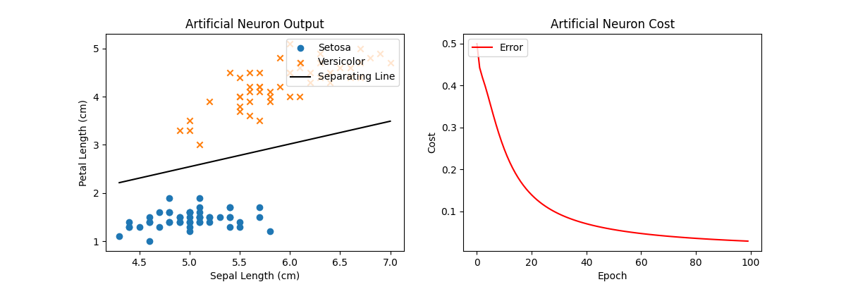
Using this new activation function and gradient descent, we’re still able to create a line separating the two classes exactly (left). The cost function on the right shows the overall cost for each iteration of gradient descent and is monotonically decreasing until it approaches 0. Note that there are more than several sets of solutions to this specific separation problem (the space between the two classes is large) so any solution that has the lowest cost will work. Intuitively, we can think of this learning problem to have a non-unique global minima or a “basin” of optimal solutions. This is often not the case with more complex problems.
One criticism is in the cost function itself. Remember that we replaced the step function with the sigmoid because it wasn’t continuous everywhere and the gradient was 0 everywhere. The derivative of the absolute value function is also not continuous everywhere, and, although the gradient does exist, it’s a constant value. Can we come up with a better cost function that provides a more well-behaved, helpful gradient? Similar to what we did with the step function, we can replace the mean absolute error cost function with a smoothed variant where the gradient not only exists everywhere, but provides a better signal on which direction to update the weights. Fortunately for us, such a function exists as the mean squared error (MSE), which just replaces the absolute value with a square.
\[C = \displaystyle\frac{1}{2}\displaystyle\sum_i \big(y_i - a_i\big)^2\]where $a_i$ is the output layer for input $x_i$. (Similar to mean absolute error, we’re adding the $\frac{1}{2}$ in front purely for mathematical convenience when computing the gradient; it’s just a constant that we could omit) This cost function is a smooth and has a derivative everywhere.
\[\begin{align*} \displaystyle\frac{\p C}{\p a_i} &= \displaystyle\sum_i -\big(y_i - a_i\big)\\ \displaystyle\frac{\p C}{\p a} &= -(y - a) \end{align*}\]Practically, smooth cost functions tend to work better since the gradient contains more information to guide gradient descent to the optimal solution. Compare this cost function gradient to the previous one that just returned $\pm 1$. In the code, we can replace the cost function and derivative with MSE instead of MAE.
def cost(pred, true):
    return 0.5 * (true - pred) ** 2

def dcost(pred, true):
    return -(true - pred)
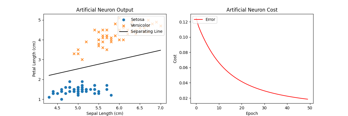
Using the new MSE cost function, we can achieve the same optimal result but notice the y-axis scale on the cost plot: it has much smaller values than that of the same plot using MAE as the cost function. This is because MSE produces very small values when true and predicted values are close but very large values when they’re farther apart. In other words, they scale with the magnitude of the difference and are not constant like with MAE.
Another point to bring up that we should address early on is efficiency of gradient descent: it requires us to average gradients over all training examples. This might be fine for a few hundred or even a few thousand training examples (depending on your compute) but quickly becomes intractable for any dataset larger than that. Rather than averaging over the entire set of training examples, we can perform gradient descent on a mini-batch that’s intended to be a smaller, sampled set of data representative of the entire training set. This is called stochastic gradient descent (SGD). We take the training data, divide it up into minibatches, and run gradient descent with parameter updates over those minibatches. An epoch still elapses after all minibatches are seen; in other words, the union of all minibatches form the entire training data, and that’s when an epoch passes. While the cost function plot to convergence is a bit noisier than full gradient descent, it’s often far more efficient per iteration since the minibatch size is much smaller. We can update the corresponding code to shuffle and partition our training data into minibatches, iterate over them, and perform a gradient descent update over the current minibatch instead of the entire training set.
class ArtificialNeuron:
    def __init__(self, input_size, learning_rate=0.5, num_epochs=50, minibatch_size=32):
        self.learning_rate = learning_rate
        self.num_epochs = num_epochs
        self.minibatch_size = minibatch_size
        self.W_ = np.zeros(input_size)
        self.b_ = 0

    def train(self, X, y):
        self.costs_ = []

        for _ in range(self.num_epochs):
            epoch_cost = 0

            # shuffle data each epoch
            permute_idxes = np.random.permutation(X.shape[0])
            X = X[permute_idxes]
            y = y[permute_idxes]

            for start in range(0, X.shape[0], self.minibatch_size):
                minibatch_cost = 0
                dW = np.zeros(self.W_.shape[0])
                db = 0
                # partition dataset into minibatches
                Xs, ys = X[start:start+self.minibatch_size], y[start:start+self.minibatch_size]
                for x_i, y_i in zip(Xs, ys):
                    # forward pass
                    a_i = self._forward(x_i)

                    # backward pass
                    dW_i, db_i = self._backward(x_i, y_i)

                    # accumulate cost and gradient
                    minibatch_cost += cost(a_i, y_i)
                    dW += dW_i
                    db += db_i
                # average cost and gradients across minibatch size
                dW = dW / self.minibatch_size
                db = db / self.minibatch_size
                # accumulate cost over the epoch
                minibatch_cost = minibatch_cost / self.minibatch_size
                epoch_cost += minibatch_cost

                # update weights
                self.W_ = self.W_ - self.learning_rate * dW
                self.b_ = self.b_ - self.learning_rate * db
            # record cost at end of each epoch
            self.costs_.append(epoch_cost)

# rest is the same
Note that we shuffle the training data each epoch so we have different minibatches to compute gradients with and update our parameters. In fact, we see any cyclical patterns in the cost function plot, it’s usually indicative of the same minibatches of data being seen over and over again.
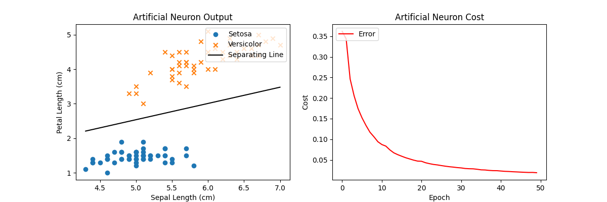
Using SGD instead of a full GD also gives an optimal solution to this problem. Note the loss curve in the right plot is noisier than using full GD since we’re randomly sampling minibatches across the training input rather than evaluating the entire training set for each iteration. In fact, in some iterations, the cost actually goes up a little bit! But the overall trend goes to 0 and that long-term trend is more important.
Now when we run the code, our loss curve looks a bit noisier but each iteration by itself is faster since we’re only using a fraction of the entire training input, yet we can still converge to a similar solution. Computing gradients over minibatches rather than the entire dataset is essential for any practical training on real-world data!
The full code listing is here.
Conclusion
In this post, we learned about numerical optimization and how we could automatically solve for the parameters of our perceptron and artificial neuron (as well as any other mathematical model, in fact!) using gradient descent. Along the way, we discovered some issues with our perceptron model, such as our step function activation, and evolved our perception into something more modern using the sigmoid activation. We also covered a few improvements for gradient descent, e.g., better choice of cost function as well as minibatching, that can help it achieve better performance in terms of speed and quality of result.
In the next post, we’ll use this neuron model as a building block to construct deep neural networks and discuss how we actually train them when they do have millions of parameters. I had originally planned to cover true artificial neural networks and backpropagation in this post as well but felt like it was already big enough to stand alone. Also backpropagation takes a lot of time and explanation that I think deserves its own dedicated article. Hopefully I turn out to be correct for next time 🙂