Restricted Boltzmann Machines

Restricted Boltzmann Machines (RBMs) are a staple for any class discussing neural networks or unsupervised learning. RBMs are essentially two-layered unsupervised stochastic neural networks that try to learn the distribution of the inputs presented to it. $\newcommand{\bigCI}{\mathrel{\text{$\perp\mkern-5mu\perp$}}}$

Make no mistake: RBMs are not easy to understand. They’re one of the most challenging topics in neural networks, and I’ve found that many explanations of RBMs that put the reader knee-deep in pages and pages of equations and theorems and proofs. As with my previous post on backpropagation, I’m going to take a more intuitive approach to explaining RBMs that avoids pages of equations but still touches on the important topics such as training and inference.

Visual Structure

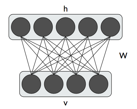
Having a visual representation of an RBM helps explain the components. An RBM has two layers: the visible layer $v$ with $D$ visible neurons/units and the hidden layer $h$ with $H$ hidden neurons/units. We also have biases for the visible and hidden units $c_k$ and $b_j$, respectively. Each visible unit is connected to each hidden unit using a single weight matrix $W$ with dimensionality $H\times D$. As the name implies, we don’t know the values of the hidden units: we only know the probability it could take on a specific value. This is the stochastic nature of the RBM. And speaking of the actual values, we’ll be discussing binary units, i.e., each hidden and visible unit can only take two values: 0 or 1.

What should the values of the hidden units be to learn the input distribution? We don’t quite know; that’s part of the training! Since we’re dealing with probabilities, it makes sense for us to use some metric that involves probabilities. Taking a page from physics, we can consider the energy of the entire configuration of visible and hidden units as the following.

\[\begin{aligned} E(v, h) &= -h^TWv - c^Tv - b^Th\\ &= -\sum_{j,k}W_{jk} h_j v_k - \sum_k c_k v_k - \sum_j b_j h_j \end{aligned}\]

By configuration, we mean the actual values of visible and hidden units. Using this notion of energy, we can compute a joint distribution for the visible and hidden units.

\[p(v, h) = \frac{1}{Z}\exp[-E(v, h)]\]

where Z is a normalizing constant that sums over all possible states: $Z=\sum_{v’,h’}\exp[-E(v, h)]$. Computing $Z$ directly is intractable. To see why, consider the case of just 10 visible neurons and 20 hidden neurons. Each neuron can take two possible values, 0 and 1, and there are 30 neurons total. This means there are $2^{30}\approx 1,000,000,000$ possible configurations and sums to compute. However, in our computations, $Z$ will usually cancel out so we don’t have to worry about it!

One interesting thing to note about this joint distribution is that low energy configurations have a higher joint probability. (Consider the shape of $f(x)=e^{-x}$.) Being in a low energy state means $h^TWv$, $c^Tv$, and $b^Th$ are large positive numbers, bringing the total energy down. In other words, the parameters are “well-aligned” with the visible and hidden units. This will become relevant when we discuss training of RBMs.

Inference

Before we discuss the algorithm used for training, let’s discuss sampling and inference assuming that our RBM is already trained. Specifically, when we perform inference, we’re actually performing conditional inference since we fix the hidden or visible units when we sample from them, i.e., we compute $p(h\vert v)$ or $p(v\vert h)$.

The RBM has an important conditional independence property as a result of its bipartite graphical structure: a visible unit $v_k$ is independent of all other visible units given all of the hidden units: $v_k\bigCI v_1,\dots,v_{k-1},v_{k+1},\dots,v_D \vert h$. To see this, think of the RBM as a Markov Random Field (or Bayesian Network). Any path from one visible unit to another always passes through a hidden unit. Similarly, a hidden unit $h_j$ is conditionally independent of all other hidden units given the visible units: $h_j\bigCI h_1,\dots,h_{j-1},h_{j+1},\dots,h_H \vert v$. This conditional independence property becomes important when we discuss Gibbs Sampling because it allows us to quickly perform block updates of the visible and hidden units.

The inference formulas are actually quite simple and elegant.

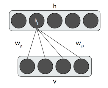
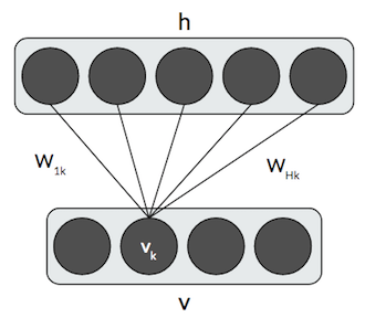
\[\begin{aligned} p(h\vert v) &= \prod_j p(h_j\vert v) \\ p(h_j=1\vert v) &= \sigma(\sum_k W_{jk} v_k + b_j) \\ p(v\vert h) &= \prod_k p(v_k\vert h) \\ p(v_k=1\vert h) &= \sigma(\sum_j h_j W_{jk} + c_k) \end{aligned}\]

where $\sigma$ is the sigmoid. In other words, the probability that a hidden unit $h_j=1$ is the sigmoid of the weighted sum of the row or column of $W$ plus a bias term. For the hidden units, we consider only the $j$th row of $W$, and, for the visible units, we consider only the $k$th column of $W$. It will become clear later why we perform inference on the visible units.

Here’s a graphical representation of how we perform conditional inference for a visible or hidden unit.

One side note on the use of the sigmoid. Do not think of this as an “activation function”! RBMs don’t actually use an activation function. The reason we have a sigmoid is because, at a step in the derivation, we have an equation of the form $\frac{1}{1+\exp(\cdot)}$, which is convenient to represent as a sigmoid. The sigmoid in these conditional inference equations is not exchangeable with another neural network activation function!

To derive the conditional inference equations, we start with the join distribution we defined above and sum out either $h$ or $v$. We also use the conditional independence property of RBMs to simplify the sum-of-sums into a single product.

Training RBMs Using Contrastive Divergence

Now that we understand the structure of an RBM, we have to figure out how to train it. We have three parameters to train: the weights, the hidden units’ biases, and the visible units’ biases. We’re going to use the principle of gradient descent and take the partial derivative of the loss function with respect to each of these parameters. (We don’t actually train RBMs using gradient descent, however; we use the (persistent) contrastive divergence algorithm, which has an additional Gibbs Sampling step.)

But what do we use as the loss function? Remember that RBMs are unsupervised models; we can’t use any supervised learning loss functions like categorical cross-entropy. Think back to the purpose of the RBM: we’re trying to learn the distribution of the inputs, i.e., the visible units. But these are stochastic, not deterministic, since the hidden units are stochastic. Learning the distribution of the inputs means we want to maximize the probability of the visible units $p(v)$. How do we compute $p(v)$ with $p(v, h)$? To compute this marginal, we simply sum out $h$. We seem to have our (pseudo-)loss function: $p(v)$!

However, probabilities aren’t usually stable or have nice derivatives. Furthermore, if we had a product of probabilities, they tend to underflow and round to zero, which is not good for training! Instead, we take the log of the probability $\ln p(v)$. This doesn’t change the overall optimization problem because $\ln(x)$ is a monotonically increasing function. Using the log-probability, for really small values of $p(v)$, we’ll simply have a really negative value, which solves our underflow problem. Also, recall that $p(v)$ and $p(v, h)$ are in terms of exponentials; taking the log of these helps “unwrap” the exponentials, and we end up with derivatives that play nice.

One additional little modification we do is add a negative sign so that we’re minimizing instead of maximizing. Many optimizers are tuned for minimization instead of maximization so adding a simple negative sign can flip a maximization problem into a minimization problem. This also changes our pseudo-loss function into a legitimate loss function, which must be nonnegative. Note that the best possible loss value of 0 occurs when $p(v)=1$, i.e., we’ve modeled the input distribution exactly.

After incorporating all of these modifications, the end result is the average negative log likelihood loss function.

\[\begin{aligned} \mathcal{L} &= \frac{1}{T} \sum_t -\ln p(x^{(t)})\\ p(x^{(t)}) &= \sum_{h\in\{0,1\}^H} \frac{1}{Z}\exp[-E(x^{(t)}, h)] \end{aligned}\]

where $x^{(t)}$ is a training example and $T$ is the training set size. Now that we have a loss function, we can compute the partial derivative of it with respect to all of our parameters. It turns out that we can compute this partial derivative with respect to a generic parameter $\theta$ and leave it in terms of $\frac{\partial E(v, h)}{\partial\theta}$ since all of the parameters are inside of the energy function.

The gradient of the negative log likelihood with respect to a parameter $\theta$ is the following.

\[\frac{\partial (-\ln p(v))}{\partial\theta} = \mathbb{E}_h\left[\frac{\partial E(v, h)}{\partial\theta}\vert v\right] - \mathbb{E}_{v,h}\left[\frac{\partial E(v, h)}{\partial\theta}\right]\]

This formulation requires some explanation. $\mathbb{E}$ is the expectation, first over all of the hidden units, i.e., the marginal distribution, then over the joint distribution, which is intractable as we’ve seen. We use expected values because the hidden units are stochastic, i.e., we don’t know the values of the hidden units to use in the computation.

The gradient consists of a positive quantity, called the positive gradient or positive phase, and a negative quantity, called the negative gradient or the negative phase. The positive gradient, a conditional expectation, is tractable; the expanded form is $\sum_h p(h\vert v)\frac{\partial E(v, h)}{\partial\theta}$, and we can compute $p(h\vert v)$ from the equation in the previous section.

However, the negative gradient is intractable since it sums over all of the visible and hidden units. The expanded form is $\sum_{v, h} p(v, h)\frac{\partial E(v, h)}{\partial\theta}$. We need to come up with a way to get around computing this intractable sum, and our answer lies in statistics.

Instead of computing the full joint expectation, let’s approximate the joint expected value with a sample taken from the joint distribution. How do we pick this sample? We use a technique from statistics called Gibbs sampling.

Gibbs Sampling

In the general case, Gibbs sampling is used in statistics to draw samples from a joint distribution of variables $S_1, S_2, \dots, S_N$. We take a random sample from the joint distribution and simply update each variable $S_i$ using the conditional probability of $S_i$ given the other variables: $S_i\sim p(S_i\vert S_{-i})$.

In the case of our RBM, $S_1, \dots, S_N$ are our visible and hidden units, and the joint distribution we’re drawing samples from is $p(v, h)$. Technically, Gibbs sampling tells us to update a given unit $v_k\sim p(v_k\vert v_1, \dots, v_{k-1}, v_{k+1}, \dots, v_D, h_1, \dots, h_H)$ one-at-a-time. But remember the conditional independence property of RBMs: a given visible unit is independent of all of other visible units given the hidden units (and similarly for the hidden units). Hence, we can update all visible units in one step, $v\sim p(v\vert h)$ and the hidden units in another step: $h\sim p(h\vert v)$.

The more steps we take, i.e., compute updates, the more accurate our final sample will be. We usually have a fixed number of steps, denoted as $\kappa$. In practice, $\kappa=1$ works well.

The following algorithm describes Gibbs sampling.

1. Initialize the visible units to the training example $v^{(0)} = x^{(t)}$ and the hidden units randomly.
2. For $\kappa$ steps do
3. Update all hidden units probabilistically according to $h^{(n+1)}\sim\sigma(W v^{(n)} + b)$
4. Update all visible units probabilistically according to $v^{(n+1)}\sim\sigma((h^{(n+1)})^T W + c)$
5. End for

(There’s a slight abuse of notation here; I define $\sigma(x)$, where $x$ is a vector, to operate independent in each component of $x$.)

In other words, $h^{(n+1)}$ is chosen to be 1 with probability $\sigma(W v^{(n)} + b)$ and 0 otherwise and similarly for the visible units. After Gibbs sampling, we get $\tilde{h} = h^{(\kappa)}$ and $\tilde{v} = v^{(\kappa)}$. We can now use these samples to replace the joint expectation and make it tractable!

Using the Gibbs Sample

Now that we have a Gibbs sample, we can actually replace the negative gradient with something simpler. In particular, let’s use $\tilde{v}$ to replace the expectation over the joint distribution with the expectation over just the hidden units.

\[\mathbb{E}_{v,h}\left[\frac{\partial E(v, h)}{\partial\theta}\right] = \mathbb{E}_{h}\left[\frac{\partial E(\tilde{v}, h)}{\partial\theta}\vert \tilde{v}\right]\]

This conveniently makes our negative gradient and positive gradient compute the expected value over the same set of units. Our new gradient looks like this.

\[\frac{\partial (-\ln p(v))}{\partial\theta} = \mathbb{E}_h\left[\frac{\partial E(v, h)}{\partial\theta}\vert v\right] - \mathbb{E}_{h}\left[\frac{\partial E(\tilde{v}, h)}{\partial\theta}\vert \tilde{v}\right]\]

Both of these expectations are tractable! Now we can use this to come up with update rules for our parameters!

Parameter Update Rules

I’d like to derive an update rule from scratch just once to show how we deal with that expectation of the partial derivative over the hidden units. We’ll compute the gradient with respect to the weight matrix $W$. We first need to compute the partial derivative of the energy function with respect to the $W$.

\[\begin{aligned} \frac{\partial E(v, h)}{\partial W_{jk}} &= \frac{\partial}{\partial W_{jk}} [-\sum_{j,k}W_{jk} h_j v_k - \sum_k c_k v_k - \sum_j b_j h_j]\\ &= -h_j v_k\\ \nabla_W E(v, h)&=-hv^T \end{aligned}\]

Now we have to compute the expectation of that partial derivative over our hidden units given the visible units. We simply apply the definition of expected value. It’s the sum over all possible values of the quantity in the expectation times the probability of those values. Since this is a conditional expectation, the probability is a conditional probability. I’ve also un-vectorized it since the hidden units are independent of each other given the visible units. (That’s the conditional independence property!)

\[\begin{aligned} \mathbb{E}_h\left[\frac{\partial E(v, h)}{\partial W_{jk}}\vert v\right] &= \mathbb{E}_h\left[-h_j v_k\vert v\right]\\ &= \sum_{h_j\in\{0, 1\}} -h_j v_k p(h_j\vert v)\\ &= -v_k p(h_j=1\vert v)\\ \mathbb{E}_h\left[\nabla_W E(v, h)\vert v\right] &= -h(v)v^T \end{aligned}\]

where $h(v)\equiv\sigma(Wv+b)$. This is a similar abuse of notation I mentioned before where the sigmoid operates on each component independently. Now we can fully incorporate this into an update rule.

\[\begin{aligned} W &\gets W - \alpha(\nabla_W -\ln p(x^{(t)}))\\ W &\gets W - \alpha(\mathbb{E}_h\left[\frac{\partial E(x^{(t)}, h)}{\partial W_{jk}}\vert x^{(t)}\right] - \mathbb{E}_{h}\left[\frac{\partial E(\tilde{x}, h)}{\partial W_{jk}}\vert \tilde{x}\right])\\ W &\gets W + \alpha(-h(x^{(t)})(x^{(t)})^T -h(\tilde{x})\tilde{x}^T) \end{aligned}\]

where $\alpha$ is the learning rate. We substitute the current example as the visible units, i.e., $v = x^{(t)}$. Since the positive and negative gradients are of the same form, we don’t have to figure out the expectation for the negative gradient. This finishes our derivation! Here are the update rules for the RBM, including the visible units’ and hidden units’ biases.

\[\begin{aligned} W &\gets W + \alpha(-h(x^{(t)})(x^{(t)})^T -h(\tilde{x})\tilde{x}^T)\\ b &\gets b + \alpha(-h(x^{(t)}) -h(\tilde{x}))\\ c &\gets c + \alpha(x^{(t)} - \tilde{x}) \end{aligned}\]

Trying going through those Now we have all we need to train our RBMs!

The Contrastive Divergence Algorithm

We’ve covered a lot in this section so I wanted to condense everything into a single, high-level algorithm to train RBMs, called Contrastive Divergence.

1. For each training example $x^{(t)}$ do
2. $\tilde{x}\gets\mathtt{Gibbs}(x^{(t)}, \kappa)$
3. $W\gets W + \alpha(-h(x^{(t)})(x^{(t)})^T -h(\tilde{x})\tilde{x}^T)$
4. $b\gets b + \alpha(-h(x^{(t)}) -h(\tilde{x}))$
5. $c\gets c + \alpha(x^{(t)} - \tilde{x})$
6. End for

where $\mathtt{Gibbs}(x^{(t)}, \kappa)$ refers to everything in the Gibbs Sampling section, i.e., alternating updates between visible and hidden units.

Persistent Contrastive Divergence

There’s one small change to the Contrastive Divergence algorithm we can make that will help our RBM get out of local minima. In the Gibbs sampling step, instead of initializing the visible units to the current sample, initialize them to the previous iteration’s Gibbs sample $\tilde{x}$, and initialize the hidden units to the previous iteration’s Gibbs sample $\tilde{h}$. This small changes helps get us out of local minima by allowing us to “wander” further from the training point $x^{(t)}$. Intuitively, when we take a Gibbs sample, we’re kind of “jumping” around the training point we’re using. There may be regions of lower energy nearby that we won’t be able to find.

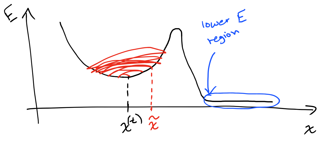
By initializing to the previous Gibbs sample, we have a better change of jumping out of local minima by “exploring” more, away from $x^{(t)}$. This is a really subtle change to Contrastive Divergence, but the research shows that this produces faster and more accurate results.

Generalizations

So far, we’ve only discussed binary units. We can extend RBMs to real-valued units by adding a quadratic term to the energy function $\frac{1}{2}v^Tv$, which changes our conditional probability function $p(v\vert h)$ to produce a Gaussian distribution instead of Bernoulli.

You were probably wondering why RBMs are called Restricted Boltzmann Machines. They are a special case of the general Boltzmann Machine. The only change is that the visible and hidden units now have lateral connections as well.

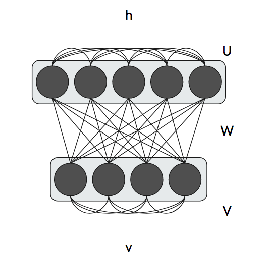
These lateral connections in the visible and hidden layer are represented as matrices $V$ and $U$ respectively. Our energy function changes to by adding quadratic terms to incorporate these lateral connections.

\[E(v, h) = -h^TWv - c^Tv - b^Th - \underbrace{\frac{1}{2}v^TVv}_{\text{visible units lateral}} - \underbrace{\frac{1}{2}h^T U h}_{\text{hidden units lateral}}\]

We have to reconsider many things, such as the partial derivatives of the energy and Gibbs sampling, to account for these new lateral connections. Boltzmann Machines are almost never used in practice because they are very difficult to train. RBMs are almost always preferred to plain Boltzmann Machines, but are still quite difficult to train.

Applications

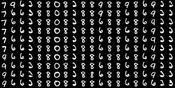
After an RBM is trained, we can sample from it using Gibbs sampling to generate new data that looks just like the training data of the RBM. For example, if we trained an RBM on the MNIST handwritten digits dataset, we can produce new handwritten digits based on the ones we’ve seen.

Source

RBMs are also the building block in deep belief networks (DBNs), which stack RBMs on top of each other for deep unsupervised learning. We have an architecture where we have a single visible layer and several hidden layers stacked on top of each other.

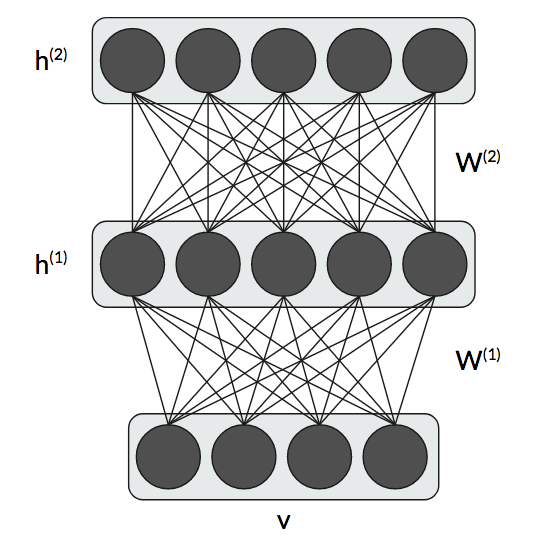
Our energy function has to incorporate two sets of weights and hidden units, and our joint probability includes all of the hidden units as well. Training one RBM was challenging enough! Training a DBN is even more challenging. But the resulting samples usually look better than a single RBM since we learn higher-level features. These have fallen out-of-style because they are so difficult to train.

The Contrastive Divergence algorithm is also used for unsupervised pre-training.

Conclusion

To summarize, Restricted Boltzmann Machines are unsupervised neural models that learn the input distribution. We train them using contrastive divergence, and, once trained, they can generate novel samples from the training dataset.

Recently, They’ve fallen out-of-style for novel data generation due to the advent of generative adversarial networks (GANs), which also learn how to generate samples from the input dataset.

I hope this post has shed some light on how and why RBMs work in a more intuitive fashion without burying you in mathematics 🙂