Language Modeling - Part 4: Transformers

In the previous post, we discussed one of the first deep learning model build specifically for language modeling: recurrent neural networks, with both plain and with long short-term memory cells. For a period of time, they were the state-of-the-art for language model as well as cross-domain tasks like image captioning. In retrospect, they did a fairly decent job at these tasks, even though they had issues with generating longer texts. We pushed these models to the limit by adding more and more parameters, making them bidirectional, and stacking them until we hit dataset and computational limits. However the beauty of research is that, every few years, a novel approach that’s a drastic departure from all previous work revolutionizes some task or subfield. The approach that did this for language modeling (and later other tangential fields) is the Transformer. This is the most widely-used neural language model underpinning large language models (LLMs) like OpenAI’s ChatGPT, Anthropic’s Claude, Meta’s Llama, and many others!

In this post, I’ll finally get to discussing the state-of-the-art neural language model: the transformer! First we’ll start by analyzing the issues with RNNs. Then we’ll introduce the transformer and deep dive into their constituent parts: position encoding, multihead self-attention, layer normalization, and position-wise feedforward networks. Finally, we’ll use an off-the-shelf pre-trained GPT2 model for language modeling!

For the direct application of transformers to language modeling, we’ll specifically be discussing decoder-only transformers which just comprised of the decoder from the original Transformers paper. The original work called the full encoder-decoder architecture a “Transformer” since it was first applied to sequence-to-sequence machine translation but modern LLMs use only the decoder part of the architecture. In reality, both use 95% of the novelty of the original Transformers paper (except for cross-attention betwen the input language and output language) but it’s an unfortunate historical point.

Transformers

RNNs and the LSTM cells we discussed last time have a few issues that make them difficult to train. The largest issue with general RNNs and their recurrence relation is the bottleneck problem: we have a single, fixed-size hidden/cell state vector that represents the accumulation of everything the RNN has seen up to the current timestep, no matter how long the input sequence is. Furthermore, traditional RNNs require sequential parsing: to compute an output at timestep $t$, we need to compute the hidden state $h_t$ which is a function of all previous hidden states and inputs. If we have a long sequence, this becomes expensive to do and limits us from training on larger corpi. As we showed last time, even with LSTM cells, RNNs still suffer from the vanishing gradient problem, albeit not as severe as in vanilla RNN cells; this makes it difficult to capture long-term semantic relationships.

RNNs support arbitrary-length sequences but compress the prior history into a finite-size hidden/cell state as we progress through the input sequence. For longer sequences, we’re trying to compress a lot of information in that hidden/cell state for the next timestep to operate on. To add some numbers to this, suppose we have an input embedding size of $256$ and a hidden/cell state of size $512$. For a sequence of just $64$ tokens, the single $512$-dimensional hidden/cell state is expected to retain $64\cdot 256=16,384$ bits of information which is a compression factor of $\frac{16,384}{512}=32$ by the end of the sequence. (Not all of these data are important so this is a worst-case analysis.) In practice, we deal with much longer sequences so it becomes progressively more and more difficult to retain important information in that small hidden/cell state, which acts as a “bottleneck” for information propagation.

The Transformer architecture (Vaswani et al. 2017) was created to help remedy these issues by fundamentally changing how we process sequential text data. Since this new architecture is such a radical departure from previous neural language model architectures, let’s define it up-front and later discuss and motivate the different parts.

The Transformer architecture from Vaswani et al. 2017 featured some interesting components: (i) a positional encoding as an efficient way to understand the relative position of tokens in the input sequence; (ii) a multihead self-attention mechanism to help retain long-term semantic relationships between tokens; (iii) layer normalization to help with regularization; (iv) a point-wise feedforward neural network to add more parameters and non-linearity; and (v) residual connections to help propagate the unedited gradient backwards to all layers at all timesteps.

We’ll be diving into the details of this neural network architecture but I want to provide a short high-level description of the different pieces and their purposes. The transformer architecture consumes a fixed-length sequence of a particular size all at once (as opposed to purely sequentially like RNNs). The first step is to embed each token of the input sequence. Then we add the positional encoding to the embedding to help the model reason about the positions of tokens and their relative relations; this is a sort of substitute for the recurrence relation. Then we apply a multihead self-attention mechanism to allow the model to dynamically focus on certain parts of the entire previous input (to help with the bottleneck problem!). We have some residual connections to help propagate the unedited gradient and some regularization to prevent overfitting. Finally, we have point-wise feedforward neural networks to process each token in the sequence in the same way and to help increase the number of parameters of non-linearity of the model.

Compare this to the RNN-based architecture to see how radically different it is! It’s a bit difficult to motivate directly but, similar to the motivation for LSTM cells, we can at least assess if we’re addressing the aforementioned issues with RNNs.

The first issue with RNN-based architectures was that we had to process the input data sequential. With the Transformer, we process the input sequence (albeit batched) all at once. This makes it much easier to chunk, parallelize, and optimize the forward and backwards passes; in fact, when we discuss the multihead attention module, we’ll see how we can optimize the operation across the entire input sequence into a single large matrix multiplication (which GPUs love!). The other issue was maintaining long-term dependencies: we’ll see later how the multihead self-attention module helps the model learn these associations by giving the model an opportunity to “attend” to all previous timesteps rather than use a condensed hidden/cell state.

With that, let’s dive into each individual module in more detail.

Positional Encoding

One of the major issue that makes RNNs difficult to train efficiently is that we have to process the input sequentially. Transformers do away with this by processing the input data in batches where the model sees the entire batch of input data at the same time. However, we lose information about the ordering of the input tokens so we need a way to bring that back.

There are two pieces to the puzzle we’ll have to solve: how to compute the embedding $\text{PE}$ and how to fold it into the input $x_t$. For the latter, we primary have a few options: (i) add, (ii) element-wise multiply, and (iii) concat. Which one we choose depends on how we compute the embedding too but let’s start very simply with addition:

\[y_t = x_t + \text{PE}_t\]

To start, the embedding $\text{PE}$ can just be a vector with the absolute position.

\[y_t = x_t + t\cdot\mathbb{1}\]

where $\mathbb{1}$ is a vector of just $1$s so we effectively just create a vector of natural numbers like $\begin{bmatrix}1\cdots 1\end{bmatrix}^T$, $\begin{bmatrix}2\cdots 2\end{bmatrix}^T$, and so on for each position $t$ where the size of the vector is the same as the size of the encoding. This absolute linear positional encoding is the simplest thing to do but has significant drawbacks. First of all, absolute positions aren’t agnostic of the sequence size: longer sequences will have larger positional encodings which creates an asymmetry for shorter sequences. It would be better to have an encoding that is sequence-size-agnostic: different lengths of sequences are treated fairly. Furthermore, we use the same value across all dimensions: each $x_t$ has the dimensionality of the embedding and using $t\cdot\mathbb{1}$ means that each value in that dimension has the same value which doesn’t really provide that much distinguishing information to the model.

Positional encodings are an open area of research but let’s see what the original Transfomer paper does. They had a novel idea about using alternating sinusoids as the values of the positional encoding. Let’s first see what their proposal is and then analyze it.

\[\begin{align*} \text{PE}_{(j, 2k)} &= \sin\frac{j}{10000^{\frac{2k}{d}}}\\ \text{PE}_{(j, 2k+1)} &= \cos\frac{j}{10000^{\frac{2k}{d}}}\\ \end{align*}\]

The positional encoding $\text{PE}$ can be considered as a matrix where the row is the position $j$ in the sequence, and the column is the value of the positional encoding. $k$ doesn’t represent the dimension: it’s just a counter so we can alternate sines and cosines. $10000$ is an arbitrary number that just needs to be significantly larger than $d$, which is the dimensionality of the encoding.

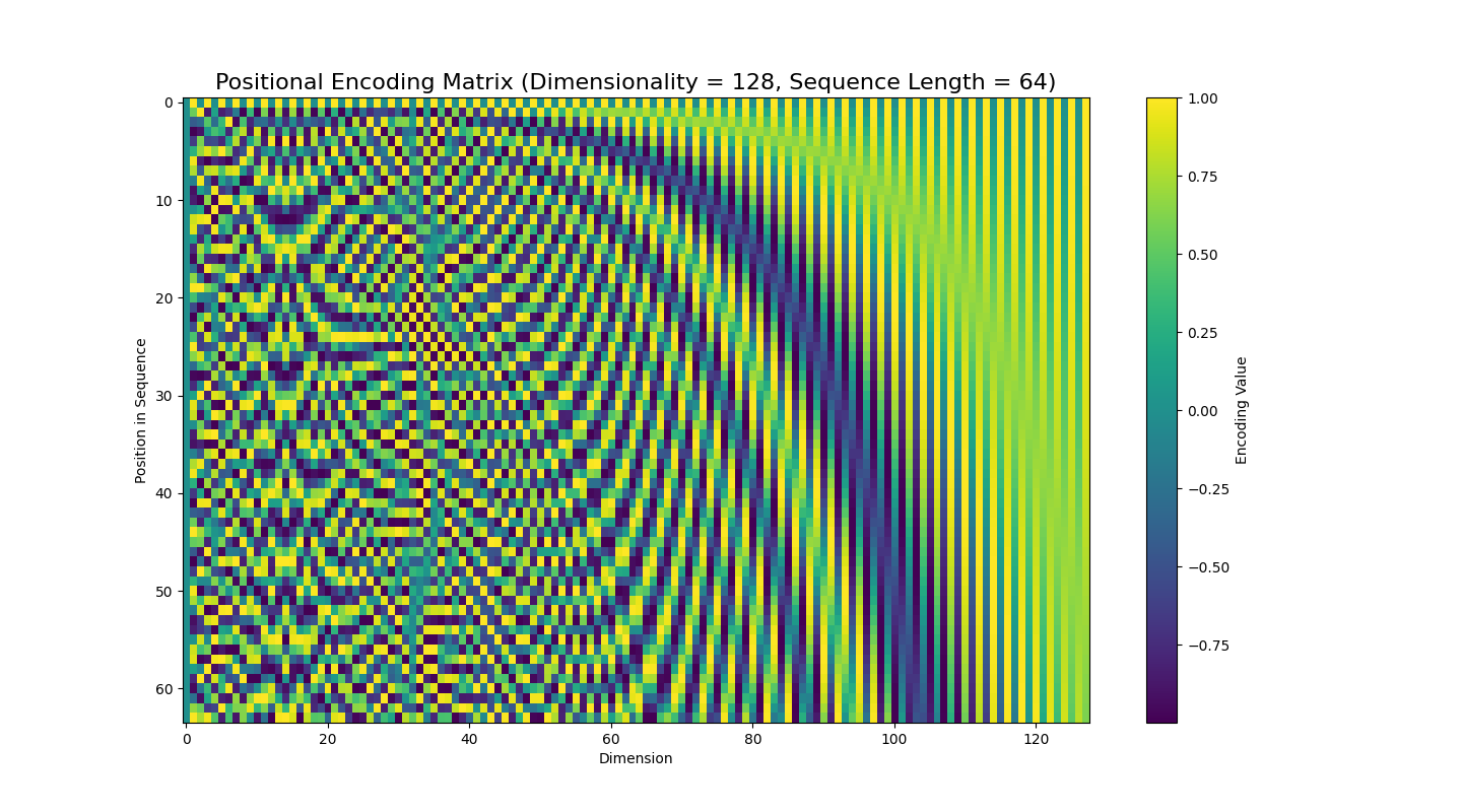
The positional encoding matrix shows how the different sinusoids blend together. In practice, we construct this for the largest forseeable sequence size and then only apply it up to the size of the sequences encountered during training. Since this is a deterministic/non-learned matrix, we can easily adapt it for larger sequence sizes if we happen to encounter one during model evaluation.

Let’s see this in action concretely with a sequence length of 4 and dimensionality of 6. The embedding can be represented by an $4\times 6$ matrix.

\[\begin{bmatrix} \sin\frac{0}{10000^{\frac{0}{d}}} & \cos\frac{0}{10000^{\frac{0}{d}}} & \sin\frac{0}{10000^{\frac{2}{d}}} & \cos\frac{0}{10000^{\frac{2}{d}}} & \sin\frac{0}{10000^{\frac{4}{d}}} & \cos\frac{0}{10000^{\frac{4}{d}}}\\ \sin\frac{1}{10000^{\frac{0}{d}}} & \cos\frac{1}{10000^{\frac{0}{d}}} & \sin\frac{1}{10000^{\frac{2}{d}}} & \cos\frac{1}{10000^{\frac{2}{d}}} & \sin\frac{1}{10000^{\frac{4}{d}}} & \cos\frac{1}{10000^{\frac{4}{d}}}\\ \sin\frac{2}{10000^{\frac{0}{d}}} & \cos\frac{2}{10000^{\frac{0}{d}}} & \sin\frac{2}{10000^{\frac{2}{d}}} & \cos\frac{2}{10000^{\frac{2}{d}}} & \sin\frac{2}{10000^{\frac{4}{d}}} & \cos\frac{2}{10000^{\frac{4}{d}}}\\ \sin\frac{3}{10000^{\frac{0}{d}}} & \cos\frac{3}{10000^{\frac{0}{d}}} & \sin\frac{3}{10000^{\frac{2}{d}}} & \cos\frac{3}{10000^{\frac{2}{d}}} & \sin\frac{3}{10000^{\frac{4}{d}}} & \cos\frac{3}{10000^{\frac{4}{d}}}\\ \end{bmatrix}\]

This seems like a fairly complicated formulation but there are several nice properties behind this. First of all, using bounded functions like sines and cosines means that this embedding is agonstic of the sequence length since it doesn’t monotonically grow (or shrink) with the length of the sequence. In the above example, we used a sequence length of 4 but, in practice, we set this to be the maximum desired sequence length and just take a slice of it for whatever sequence length we get as input. Another very nice property for the gradient is that these are mathematically smooth (continuous and infinitely differentiable) so we don’t have to worry about sparse or constant gradients.

One other important property is that using periodic functions like sines and cosines help us with learning relative positions at different scales. To explain this better, consider the most generic form of sine function:

\[f(x) = A\sin(T(x+\phi)) + b\]

where

• $A$ is the amplitude
• $\frac{2\pi}{T}$ is the period
• $\phi$ is the phase/horizontal shift ($\phi > 0$ means the plot shifts right; otherwise it shifts left)
• $b$ is the vertical shift ($b > 0$ means the plot shifts up; otherwise it shifts down)

Another useful trigonometric property is that $\sin(\theta)=\cos(\frac{\pi}{2}-\theta)$ and $\cos(\theta)=\sin(\frac{\pi}{2}-\theta)$ so we can think of sine and cosine as just being phase shifts of each other by $\frac{\pi}{2}$. Going back to the sinusoidal positional encoding, let’s just consider the even terms (knowing that the odd terms are just offset by a phase shift).

\[\text{PE}_{(j, 2k)} = \sin\frac{j}{10000^{\frac{2k}{d}}}\\\]

For this term, $A=1$ and $b=1$ so the amplitude is $1$ and there’s no vertical shift but what about the period and phase shift? Well even if we expand the $\sin$ argument, there’s no additive term, only the factor on $j$. Let’s start by holding $k$ constant and varying only $j$. This simplifies the equation into $\sin\frac{j}{c}$ where $c$ is constant; the period of this function is $2\pi c$ which we can see if we rewrite as $\sin\frac{1}{c}j$. As we progress through the sequence, the value of $j$ increases along the sinusoid.

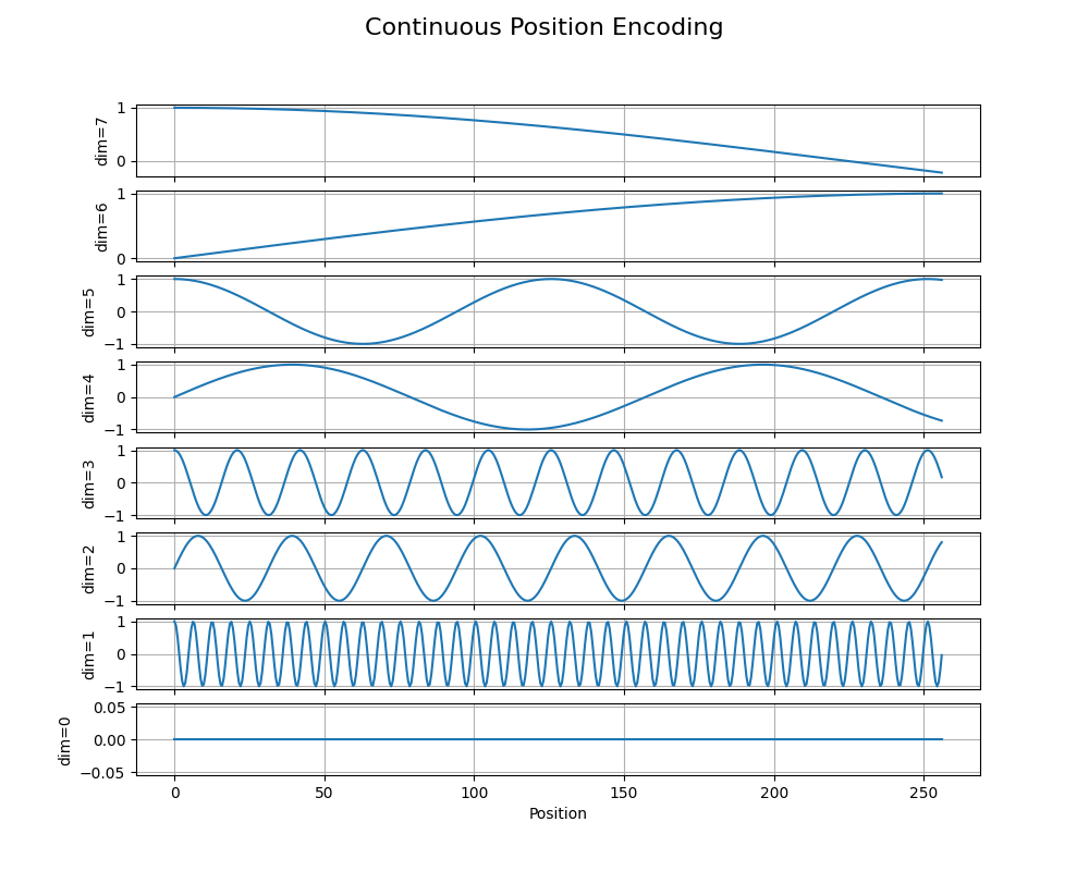
To get a better idea of the shape of the positional encoding, we can plot the positional encoding with the position in the continuous domain and the dimension in the discrete domain. As the dimension increases in pairs, the frequency of the sinusoid across the position decreases which gives the model many different ways to correlate the relative positions of different words in the input sequence. (These plots are generated from here.)

Now let’s try holding $j$ constant and varying $k$; in other words, for a particular timestep $j$, how do the values of the sinusoidal positional encoding change as the dimensionality of the embedding increases? This one is a bit trickier since $k$ is in an exponent in the denominator but we can reason about that term $10000^{\frac{2k}{d}}$. As we increase $k$, $10000^{\frac{2k}{d}}$, i.e., the denominator, increases which means the $\sin$ argument decreases. Specifically, the overall period $2\pi c$ decreases as $k$ increases: in other words, as the dimensionality of the embedding increases, the period of the sinusoids increases at a fixed timestep.

The perodicity of this encoding means that there’ll be tokens in the input that end up with the same positional encoding value at different intervals. Intuitively, this means that our model can learn relative positions of input tokens because of the repeating pattern of sinsusoids. Since the frequency increases with the dimensionality, input tokens get multiple relative positions associations for different intervals or scales.

In concrete implementations of the positional encoding, rather than seeing that exact formula above, we tend to see this formulation:

\[\text{PE}_{(j, 2k)} = \sin \Bigg[j\exp\Bigg(\frac{-2k}{d}\log{10000}\Bigg)\Bigg]\]

This modified formulation is more numerically stable since we’re taking the log of a large number instead of raising a large number to a large power (thus maybe overflowing). To get from the original formulation to the current one, take the exponential log of the quantity $10000^{-\frac{2k}{d}}$ (which is legal since the exponential log of any quantity is the quantity itself, much like adding and subtracting $1$ cleverly) and simplify until it looks like the exponential term in the above equation.

Interesting, there have been a few recent work that show the positional encoding is optional and that transformers without such encoding can perform as well as those without it. Positional encodings (or potentially lack of) still a very active area of research!

Multihead Self-Attention

The next module in the transformers architecture is multihead self-attention. This is a different flavor of an attention mechanism. To motivate it, consider an RNN language model with a long context window: as we move along the sequence, the only information we pass forward to the next timestep is the hidden/cell state. If we have a long sequence, this hidden/cell state has the huge responsibility of retaining all of the “important” information from all previous timesteps to provide to the current timestep. With an LSTM cell, the model can do a much better at determining and propagating forward the “important” information but, for longer sequence, we’re still bound by the dimensionality of the cell state; we can try increasing the size of the cell state but that adds computational complexity.

The novelty behind the attention mechanism is to reject the premise that the current timestep can only see this condensed hidden/cell state from the previous timestep. Instead, the attention mechanism gives the current timestep access to all previous timesteps instead of just the previous hidden/cell state!

The trick becomes how to integrate all previous timesteps into the current one, especially since we have a variable number of previous timesteps as we progress through the sequence. The novel contribution of self-attention is to take an input sequence and, for each timestep, numerically compute how much we should consider each previous timestep into the current one.

For each timestep, we learn a key, query, and value. Then we compute how much a query aligns with each key. This alignment is passed through a softmax layer to normalize the raw values into attention scores. Then we can multiply these against the values to figure out how much we should weigh the values when computing the current state.

Suppose the input $X$ is a matrix of $n\times d$ where $n$ is the sequence length and $d$ is the dimensionality of the embedding space. Using fully-connected layers (omitting biases for brevity), we project $X$ into three different spaces: query, key, and value:

\[\begin{align*} Q &= W_Q X\\ K &= W_K X\\ V &= W_V X\\ \end{align*}\]

We’re applying these three to all vectors in the sequence simultaneously as a vectorized operation. The key and query have the same dimension of $d_k$ while the values have a dimension of $d_v$. Now we take the dot product of each key with each value and run it through a softmax and scale it by $\sqrt{d_k}$ to get attention scores. Intuitively, these scores tell us, for a particular timestep, how much we should consider the other timesteps. We use these attention scores by multiplying them with the learned values to get the final result of the self-attention mechanism.

\[\text{Attention(Q, K, V)} = \text{softmax}\Bigg(\frac{QK^T}{\sqrt{d_k}}\Bigg)V\]

Let’s double-check the dimensions. $Q$ is $n\times d_k$ (a query vector for each input token) and $K$ is $n\times d_k$ (a key vector for each input token) so $QK^T$ is $n\times n$, and, after softmaxing across each row and scaling by $\sqrt{d_k}$, we get the attention scores that measure, for each timestep, how much we should focus on another term in the same sequence. This particular flavor is sometimes called scaled dot-product attention. We multiply these by the learned values of size $n\times d_v$ so the output will be the same.

The reason for the $\sqrt{d_k}$ is that the authors of the original Transformers paper mentioned that the dot products will get larger as the dimensionality of the space gets larger since we’re adding up element-wise products and we’ll have more terms in the sum with a larger embedding key-query dimension. (Just like with absolute positional encodings!)

To summarize, given a particular input, we map it to a key, query, and value using a fully-connected layer. Then we take the dot product of the query with each key; an intuitive way to interpret the dot product is measuring the “alignment” of two vectors. Then we can run that result through a softmax to get a probability distribution over all previous keys to multiply by the learned values to get the result of the attention module.

Instead of using a single key, query, value set, we can use multiple different ones so that the model can learn to attend to different kinds of characteristics in the input sequence. The idea is that we can copy-and-paste the same self-attention into several different attention heads using another projection, concatenate the results of all of the attention heads, then finally run the concatenation through a final fully-connected layer. This is called multi-head attention.

For multi-head self-attention we take the same self-attention mechansim with the same input but use a different set of key, query, and value weights for each head.

Mathematically, for each head, we can take a query $Q$, key $K$, and value $V$, project them again (again ignoring biases for brevity), and compute attention.

\[\text{head}^{(i)} = \text{Attention}(W_Q^{(i)}Q, W_K^{(i)}K, W_V^{(i)}V)\]

Then we can concatenate all of the heads together and project again to the the result of multihead self-attention.

\[\text{Multihead}(Q, K, V) = \Big(\text{head}^{(1)} \oplus \cdots \oplus \text{head}^{(h)}\Big)W_O\]

where $h$ represents the number of heads. We usually set $d_k=d_v=\frac{d_m}{h}$ so that we can cleanly split and rejoin the different heads without having to worry about fractional dimensions.

Now we finally have the full multi-head self-attention in the paper!

One important aspect when training this module is the causal mask $M$: it sees the entire sequence at once and computes attention scores across the whole sequence. However, this isn’t entirely accurate since, at a timestep $t$, we’ve only seen tokens at the $(1,\cdots,t-1)$ timesteps, not the entire sequence. So in the attention score matrix, we need to mask out all future timesteps using causal mask. Since a sequence is already ordered, the mask is an upper-triangular matrix with $\infty$ in the upper triange and $0$ everywhere else.

\[M=\text{Upper}(\infty)=\begin{bmatrix} \infty & \infty & \infty & \cdots & \infty\\ 0 & \infty & \infty & \cdots & \infty\\ 0 & 0 & \infty & \cdots & \infty\\ \vdots & \vdots & \vdots & \ddots & \vdots\\ 0 & 0 & 0 & \cdots & \infty\\ \end{bmatrix}\]

When we add this mask to the attention score matrix, it nullifies future tokens at each timestep so the model doesn’t cheat by “seeing into future”.

Layer Normalization

The next step in the transformer architecture is a module called Layer Normalization. In the context of neural networks, normalization is the act of perturbing the inputs to a layer with the intent to help the model generalize better and learn faster. As we train a deep neural network, the intermediate activations go through layer after layer, and each layer can have drastically different weights; if we think about the activations as a distribution, they go through many different distributional changes that the model has to exert effort in learning. This problem is called the internal covariate shift. Wouldn’t it be easier if we innocently standardized the activations before each layer? That’s exactly what normalization does! This means the model can handle different kinds of input “distributions” and doesn’t have to waste effort in learning each of the distributional shifts across layers. There are a number of other reasons why we use normalization in neural networks but this is one of the most important reasons.

There are a few different kinds of normalization but the one that’s used by the transformers paper is Layer Normalization. The idea is to normalize the values across the feature dimension. So for each example in a batch of inputs, we take the mean and variance of the features per example to get 2 scalars and then standardize each component of the input by that mean and variance, i.e., we’re shifting the “location” of the input distribution. Additionally, we also learn a scale and bias factor per feature to alter the shape of the distribution.

Given a sequence of training examples, per example, we compute a mean and variance and offset the values for that particular example. Another normalization technique popular for non-sequential data is batch normalization where we do effectively the same thing, but across a particular feature dimension in the batch instead of across the training example itself.

Suppose we have an example $x$ in the batch where each is a $d$-dimensional vector and $x_j$ is the $j$th component. First, we compute a mean $\mu$ and variance $\sigma^2$ of each example $x_i$ over its features.

\[\begin{align*} \mu &= \frac{1}{d}\sum_{j} x_{j}\\ \sigma^2 &= \frac{1}{d}\sum_j (x_{j} - \mu)^2 \end{align*}\]

Now, for each example, we offset it by its mean and standard deviation.

\[\hat{x_j} = \frac{x_j-\mu}{\sqrt{\sigma^2 + \epsilon}}\]

where $\epsilon$ is a small value for numerical stability to avoid divide by zero issues. Finally, we apply learnable scale $\gamma_j$ and shift $\beta_j$ parameters for each feature/component.

\[y_j = \gamma_j \hat{x_j} + \beta_j\]

Layer normalization helps perturb the layer activations for better training results. We apply these layers after every major component, specifically the multihead self-attention module and the position-wise feedforward network that we’ll discuss shortly!

Position-wise Feedforward Network

To help add more parameters and nonlinearity to increase the expressive power of the transformer, we add a position-wise feedforward network. It’s a little two-layer neural network that sends a vector at a single position in the sequence to a latent space and then back to the same dimension using a ReLU nonlinearlity in the middle.

\[\text{FFN}(x) = W_2\cdot\text{ReLU}(W_1x + b_2) + b_2\]

We apply this to each timestep (or position) in the sequence, hence the “position-wise” part, and it’s the same network operating on all positions independently so they operate on the input consistently.

Training

Training a transformer for language modeling is identical to training any other kind of neural model for language model. We take the raw input text and try to get the transformer to predict the next token at each timestep and use the cross-entropy loss. Remember to apply the causal mask!

GPT2

Now that we’ve grasped the basics of the core transformer architecture, let’s talk about some specifics of the OpenAI GPT2 model since the research, model weights, and tokenizer are all public artifacts! Besides the transformer architecture itself, on either ends of it are the encoding, turning raw text into a sequence of tokens for the input layer of the transformer, and decoding, producing a sequence of tokens for the tokenizer to convert back into raw text.

Byte-pair Encoding (BPE)

So far, we’ve skirted around the topic of tokenization by splitting our corpus into individual characters but that character-based representation is too local to meaningfully represent the English language. When we think about words in English, the smallest unit of understanding is called a morpheme in linguistics, and it’s often comprised of multiple characters. For example, the word “understanding” in the previous sentence is made up of two morphemes: (i) the root “understand” and (ii) the present participle “ing” meaning “in the process of”. In both cases, each morpheme is built from several characters (also called a grapheme) so using our character-level representation is not quite the right level of abstraction.

This might seem like the “magical” solution to all of our tokenization woes! Instead of coming up with any kind of tokenization scheme, let’s just take each morpheme in the English language, assign it a unique ID, and split words based on these morphemes! Unfortunately, there are several reasons this won’t just work. First of all, there are too many English morphemes! As a rough calculation, we can multiple the number of English roots with the number of affixes (like “un” and “ing”) with the number of participles and so on to arrive at about 100,000 morphemes which is a huge embedding space! Even cutting that in half to 50,000 is still a pretty large embedding! But that’s just English, other languages may have even more! Furthermore, language is an ever-evolving structure so the current set of morphemes might not be sufficient for new words; traditionally, we’d just reserve a token like <UNK> to represent unknown words in the vocabulary but that’s an extreme. New words usually don’t come out of nowhere: their constituent parts are usually from existing words.

One kind of encoding that GPT2 and others use is Byte-pair encoding (BPE): a middle-ground that tries to balance grouping graphemes into morphemes while also trying to bound the vocabulary size. Conceptually, BPE computes all character-level bigrams in the corpus and finds the most common pair, e.g., (A, B) ; then it replaces that pair with a unique token, e.g., (AB). Then we repeat the process until we reach the desired vocabulary size or there are no more character-level bigrams to merge. The trick is that we don’t use Unicode characters but actually use bytes (hence the “byte” in byte-pair encoding!).

Let’s use a dummy corpus as an example.

• m o r p h e m e
• e m u l a t o r
• l a t e r

In the first step, let’s compress e and m into a single token em.

• m o r p h em e
• em u l a t o r
• l a t e r

Now we can merge l and a into la.

• m o r p h em e
• em u la t o r
• la t e r

We can merge o and r into or.

• m or p h em e
• em u la t or
• la t e r

Then we can merge la and t into lat.

• m or p h em e
• em u lat or
• lat e r

Now there are no more character-level bigrams to merge so the vocabulary is m, or, p, h, em, e, u, lat, or, and r. Now suppose we encounter a new word like grapheme; we can partially tokenize it into [UNK r UNK p h em e] which is better than just replacing the whole word with <UNK>. This is a very simple example but it illustrates how BPE gives us a robust representation somewhere between characters and words. In reality, the vocabularies are large enough that we’d rarely have unknown sub-morphemes.

Let’s code an example using the off-the-shelf GPT2 tokenizer. (Make sure you have the transformers Python package installed!)

from transformers import GPT2TokenizerFast

tokenizer = GPT2TokenizerFast.from_pretrained('gpt2')
prompt = 'Tell me what the color of the sky is.'
tokens = tokenizer(prompt, return_tensors='pt').input_ids
print(f'Input: {prompt}\nTokens: {tokens}')

# Input: Tell me what the color of the sky is.
# Tokens: [[24446, 502, 644, 262, 3124, 286, 262, 6766, 318, 13]]

Our input prompt features words frequent enough that each entire word (and the punctuation) is represented as a whole token! Try using more complicated words or made-up words to see what the tokens would look like!

Decoding

The last stage before de-tokenizing is decoding. Recall that language models are probabilistic and compute the likelihood of a sequence of tokens. When we discussed n-gram and RNN models, we generated text using a random sampling approach where we sample the next word according to the next word’s probability distribution conditioned on the entire previous sequence, i.e., $w_t\sim p(w_t\vert w_1,\dots,w_{t-1})$.

Top-$k$ Sampling

The issue with random sampling is that we give some tiny weight to words that wouldn’t create a cohesive sentence. For example, if we had a sentence like “The cat sat on the “, there would be a nonzero likelihood of sampling “adversity”.

Rather than using the entire distribution, we should disqualify these low-likelihood words and only select the most likely ones. One way to accomplish this is to select only the $k$ most likely words, renormalize that back into a probability distribution, and sample from that distribution instead. This is called top-$k$ sampling! The intent is to remove any low-likelihood words so that it’s impossible to sample them.

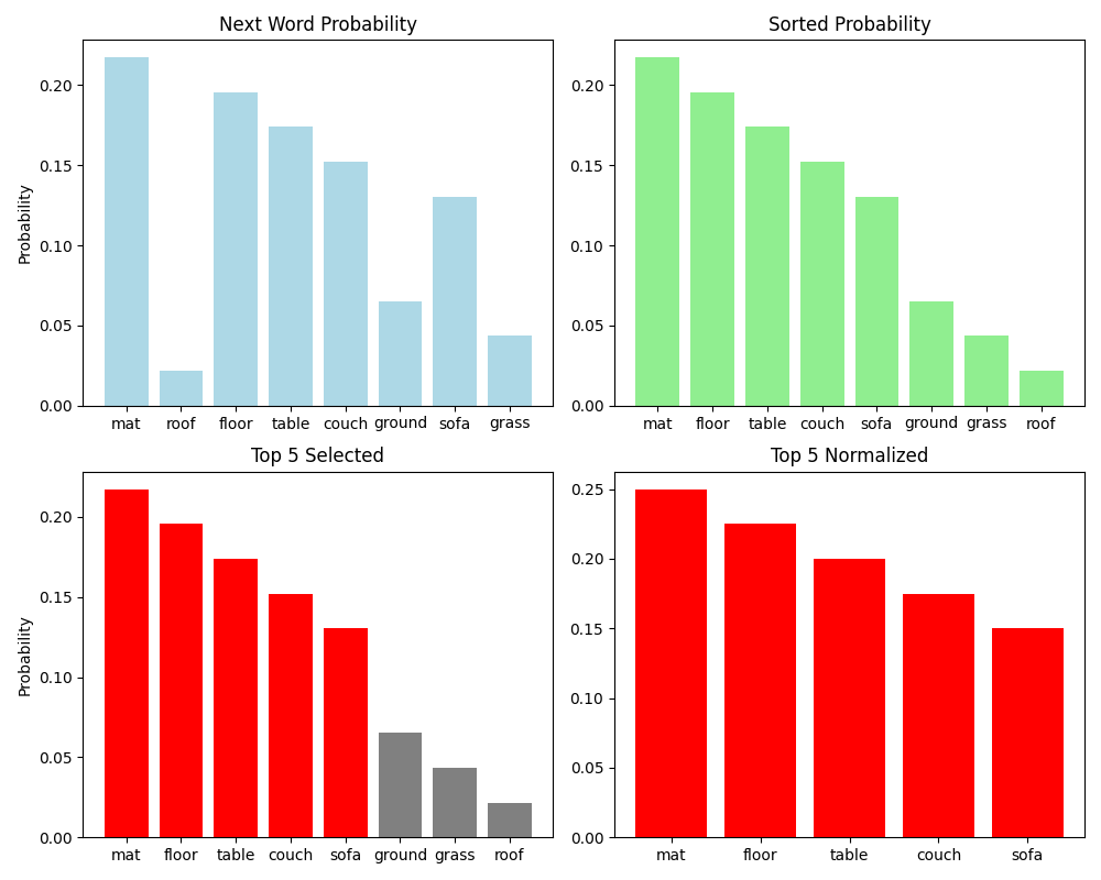
Visually, we can conceptualize it as taking the distribution $p(w_t\vert w_1,\dots,w_{t-1})$, sorting it by probability, selecting the top $k$ most likely words, renormalizing that back into a probability distribution, and sampling from that top-$k$ distribution..

When $k=1$, we recover greedy sampling where we always select the most likely word next. We can use the same transformers library to pull the GPT2 language model weights, sample using top-$k$ sampling, and de-tokenize!

from transformers import GPT2TokenizerFast, GPT2LMHeadModel

model_name = 'gpt2'
tokenizer = GPT2TokenizerFast.from_pretrained(model_name)
model = GPT2LMHeadModel.from_pretrained(model_name)

prompt = 'Some example colors are red, blue, '
model_input = tokenizer(prompt, return_tensors='pt')

# do_sample samples from the model
# no_repeat_ngram_size puts a penalty on repeating ngrams
# early_stopping means to stop after we see an end-of-sequence token
output = model.generate(**model_input, do_sample=True, top_k=10, no_repeat_ngram_size=2, early_stopping=True)

decoded_output = tokenizer.batch_decode(output, skip_special_tokens=True)
print(decoded_output)

Try it out with different values of $k$!

Top-$p$ Sampling / Nucleus Sampling

The issue with top-$k$ sampling is that $k$ is fixed across all contexts: in some contexts perhaps the probability distribution is very flat where the top $k$ words are equally likely as other words. But what if we have a probability distribution that’s heavily peaked? In that case, $k$ might still consider very unlikely words.

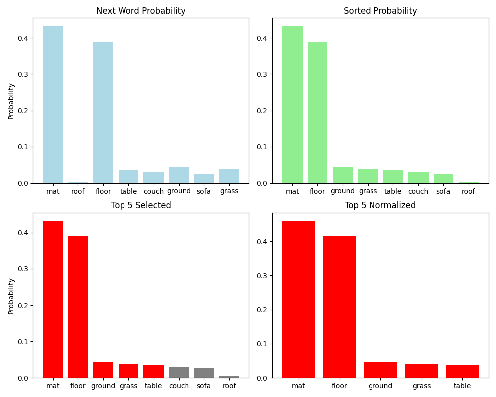
Consider this peaked distribution. Setting the wrong value of $k$ would still select unlikely words. The root of the issue is that the value of $k$ is fixed: for one word, we might get a “good” distribution but for the immediate next word, we might get this peaked distribution!

The Curious Case of Neural Text Degeneration by Holtzman et al. took a different approach: rather than selecting and sorting in the word space, they do something similar in the cumulative probability space. The idea is similar to top-$k$ in that we sort the probability distribution, but then, instead of selecting a fixed $k$ words, we select words, from the most likely to the least likely, until their cumulative probability exceeds a certain probability $p$. Think of it as having a “valid” set of words that we populate based on the cumulative probability of the set: we add the most likely word, then the next likely word, and keep going until the total probability of the set exceeds $p$. Then we stop, renormalize, and sample from that distribution.

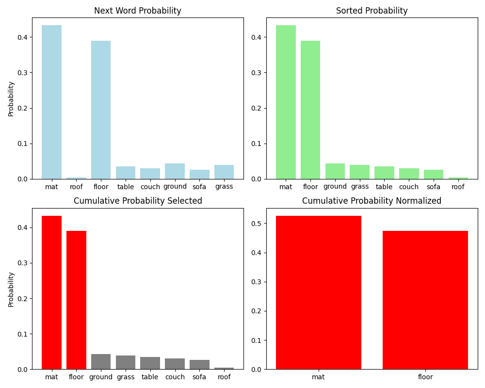
Visually, we can conceptualize it as taking the distribution $p(w_t\vert w_1,\dots,w_{t-1})$, sorting it by probability, selecting the set of words from the most likely to the least likely until the sum of their probabilities meets the threshold. Then we renormalize that back into a probability distribution and sample from that.

This overcomes the challenge of selecting the “right” $k$ value in top-$k$ sampling because we’re dynamically choosing how many words we put into the “valid” set based on what the distribution over the next word looks like. When $p$ is small, the “valid” set tends to be smaller since it takes fewer words to reach the $p$ value; this tends to produce more predictable and less diverse output. When $p$ is larger, we need more words in the “valid” set to reach the $p$ value; this tends to produce less predictable but diverse outputs. Similar to top-$k$ sampling, we can use the same transformers library to pull the GPT2 language model weights, sample using top-$p$ sampling, and de-tokenize!

# use top_p instead
output = model.generate(**model_input, do_sample=True, top_p=0.9, no_repeat_ngram_size=2, early_stopping=True)

Try it out with different $p$ values!

Temperature Sampling

One more approach to decoding is called temperature sampling because it’s inspired from thermodynamics: a system of particles at a high temperature will behave more unpredictably than one at a lower temperature. Temperature sampling mimics that behavior through a temperature parameter $\tau$. The idea is that we scale the raw logit activations $a$ by the temperature before taking the softmax: $\text{softmax}(\frac{a}{\tau})$. To understand the effect of $\tau$, recall that taking the softmax of a set of logits will tend to drive them to the extremes of 1 and 0 so if we drastically increase the value of one of the logits will increase the probabilities to the higher-likelihood words and lower the probabilities of the lower-likelihood words.

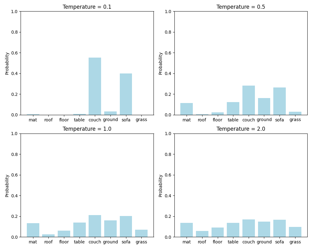
Given a distribution, lower temperatures tend to cause the distribution to be more sharply peaked towards just the few high-likelihood words; this reduces variability in the output. As the temperature gets higher, the distribution gets flatter.

Now let’s consider the role of $\tau$: if $\tau=1$, then we don’t change the distribution at all. However, for a low temperature $\tau\in(0, 1]$, we’ll increase all of the logits, thus driving the softmax distribution to high likelihood words so the sampling is more predictable (just like with lower temperature in thermodynamics!). For a high temperature $\tau > 1$, we’re making each of the logits smaller which “flattens” the distribution so it’s more likely that previously low-likelihood words would be selected which gives us more variability in the output.

Just like with the previous sampling, let’s try it out!

output = model.generate(**model_input, do_sampling=True, temperature=1.5, no_repeat_ngram_size=2, early_stopping=True)

Try playing around with different temperatures!

Conclusion

In this post, we finally arrived at the state-of-the-art neural language model: the transfomer! To better motivate the pieces, we first discussed the pitfalls of RNNs. Then we discussed the pieces of the transformers starting with the positional encoding, then moving onto multihead self-attention, through the layer norm, and finally to the position-wise feedforward networks. Finally, we used a pre-trained GPT2 language model for language modeling and discussed the encoding and decoding on either ends of the transformer to fully-construct a language model for text generation!

That’s the conclusion (?) on our tour of language modeling! We started learning about n-gram models all the way through transformers used in state-of-the-art large language models. Most of what I’ve seen now is people using LLMs to build really cool creative things, but I hope this tour has helpee peel back the curtain behind how they work 🙂